obspy.realtime.rttrace.RtTrace.remove_response¶

RtTrace.remove_response(inventory=None, output='VEL', water_level=60, pre_filt=None, zero_mean=True, taper=True, taper_fraction=0.05, plot=False, fig=None, **kwargs)¶

Deconvolve instrument response.

Uses the adequate obspy.core.inventory.response.Response from the provided obspy.core.inventory.inventory.Inventory data. Raises an exception if the response is not present.

Note that there are two ways to prevent overamplification while convolving the inverted instrument spectrum: One possibility is to specify a water level which represents a clipping of the inverse spectrum and limits amplification to a certain maximum cut-off value (water_level in dB). The other possibility is to taper the waveform data in the frequency domain prior to multiplying with the inverse spectrum, i.e. perform a pre-filtering in the frequency domain (specifying the four corner frequencies of the frequency taper as a tuple in pre_filt).

Note

Any additional kwargs will be passed on to obspy.core.inventory.response.Response.get_evalresp_response(), see documentation of that method for further customization (e.g. start/stop stage).

Note

Using remove_response() is equivalent to using simulate() with the identical response provided as a (dataless) SEED or RESP file and when using the same water_level and pre_filt (and options sacsim=True and pitsasim=False which influence very minor details in detrending and tapering).

Example

>>> from obspy import read, read_inventory
>>> st = read()
>>> tr = st[0].copy()
>>> inv = read_inventory()
>>> tr.remove_response(inventory=inv)  
<...Trace object at 0x...>
>>> tr.plot()  

(Source code, png, hires.png)

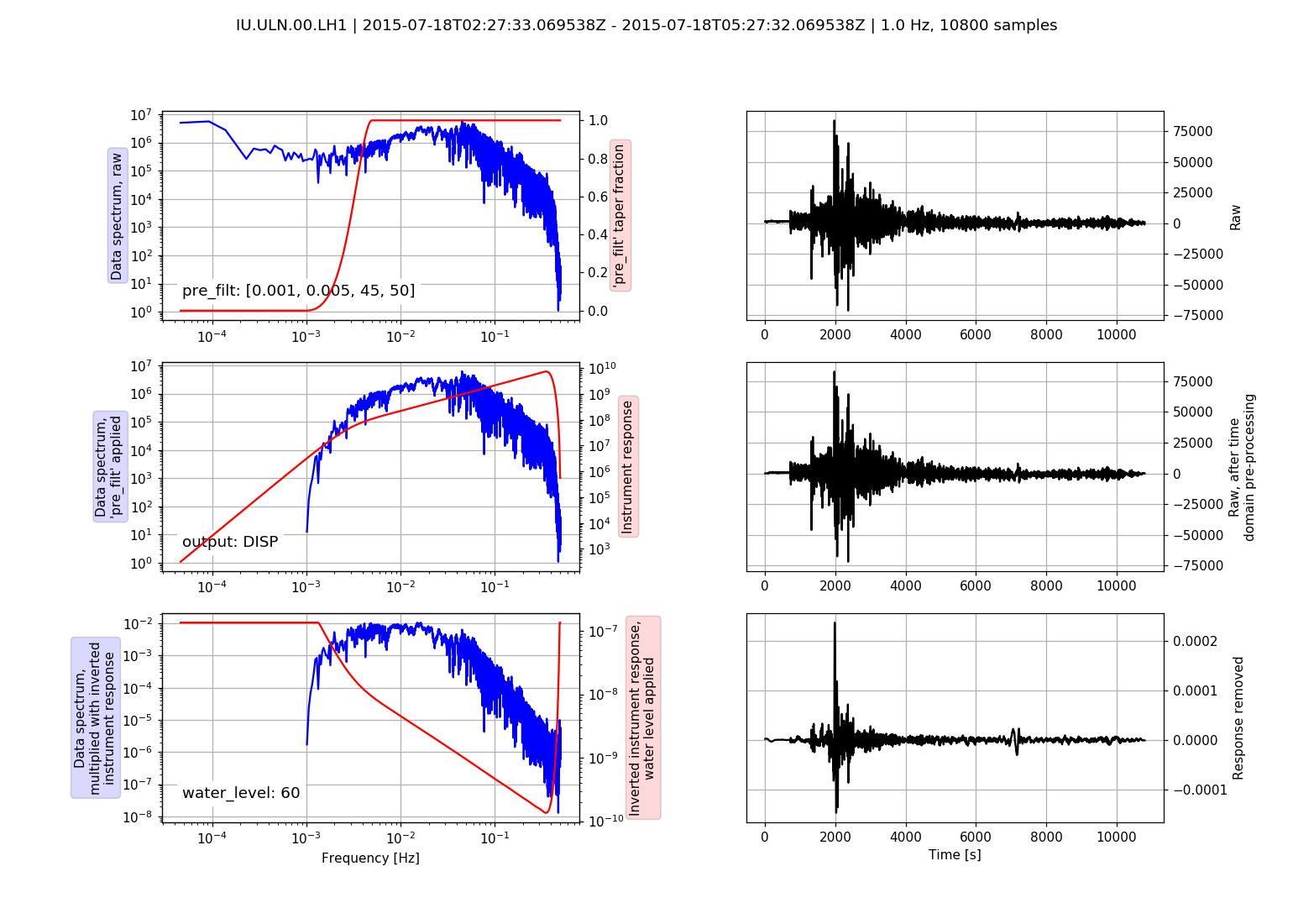
Using the plot option it is possible to visualize the individual steps during response removal in the frequency domain to check the chosen pre_filt and water_level options to stabilize the deconvolution of the inverted instrument response spectrum:

>>> from obspy import read, read_inventory
>>> st = read("/path/to/IU_ULN_00_LH1_2015-07-18T02.mseed")
>>> tr = st[0]
>>> inv = read_inventory("/path/to/IU_ULN_00_LH1.xml")
>>> pre_filt = [0.001, 0.005, 45, 50]
>>> tr.remove_response(inventory=inv, pre_filt=pre_filt, output="DISP",
...                    water_level=60, plot=True)  
<...Trace object at 0x...>

(Source code, png, hires.png)

Parameters:

inventory (Inventory or None.) Station metadata to use in search for adequate response. If inventory parameter is not supplied, the response has to be attached to the trace with Trace.attach_response() beforehand. output (str) Output units. One of: "DISP" displacement, output unit is meters "VEL" velocity, output unit is meters/second "ACC" acceleration, output unit is meters/second**2 water_level (float) Water level for deconvolution. pre_filt (list or tuple of four float) Apply a bandpass filter in frequency domain to the data before deconvolution. The list or tuple defines the four corner frequencies (f1, f2, f3, f4) of a cosine taper which is one between f2 and f3 and tapers to zero for f1 < f < f2 and f3 < f < f4. zero_mean (bool) If True, the mean of the waveform data is subtracted in time domain prior to deconvolution. taper (bool) If True, a cosine taper is applied to the waveform data in time domain prior to deconvolution. taper_fraction (float) Taper fraction of cosine taper to use. plot (bool or str) If True, brings up a plot that illustrates how the data are processed in the frequency domain in three steps. First by pre_filt frequency domain tapering, then by inverting the instrument response spectrum with or without water_level and finally showing data with inverted instrument response multiplied on it in frequency domain. It also shows the comparison of raw/corrected data in time domain. If a str is provided then the plot is saved to file (filename must have a valid image suffix recognizable by matplotlib e.g. ‘.png’).