20. Basemap Plots
20.1. Basemap Plot with Custom Projection Setup
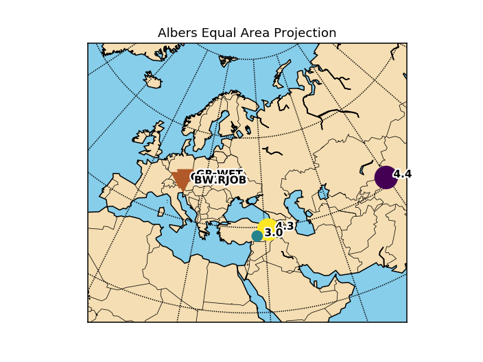
Simple Basemap plots of e.g. Inventory or Catalog objects can be performed with builtin methods, see e.g. Inventory.plot() or Catalog.plot().
For full control over the projection and map extent, a custom basemap can be set up (e.g. following the examples in the basemap documentation), and then be reused for plots of e.g. Inventory or Catalog objects:
from mpl_toolkits.basemap import Basemap
import numpy as np
import matplotlib.pyplot as plt

from obspy import read_inventory, read_events

# Set up a custom basemap, example is taken from basemap users' manual
fig, ax = plt.subplots()

# setup albers equal area conic basemap
# lat_1 is first standard parallel.
# lat_2 is second standard parallel.
# lon_0, lat_0 is central point.
m = Basemap(width=8000000, height=7000000,
            resolution='c', projection='aea',
            lat_1=40., lat_2=60, lon_0=35, lat_0=50, ax=ax)
m.drawcoastlines()
m.drawcountries()
m.fillcontinents(color='wheat', lake_color='skyblue')
# draw parallels and meridians.
m.drawparallels(np.arange(-80., 81., 20.))
m.drawmeridians(np.arange(-180., 181., 20.))
m.drawmapboundary(fill_color='skyblue')
ax.set_title("Albers Equal Area Projection")

# we need to attach the basemap object to the figure, so that obspy knows about
# it and reuses it
fig.bmap = m

# now let's plot some data on the custom basemap:
inv = read_inventory()
inv.plot(fig=fig, show=False)
cat = read_events()
cat.plot(fig=fig, show=False, title="", colorbar=False)

plt.show()
(Source code, png, hires.png)

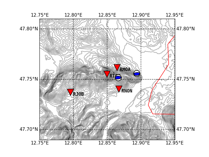
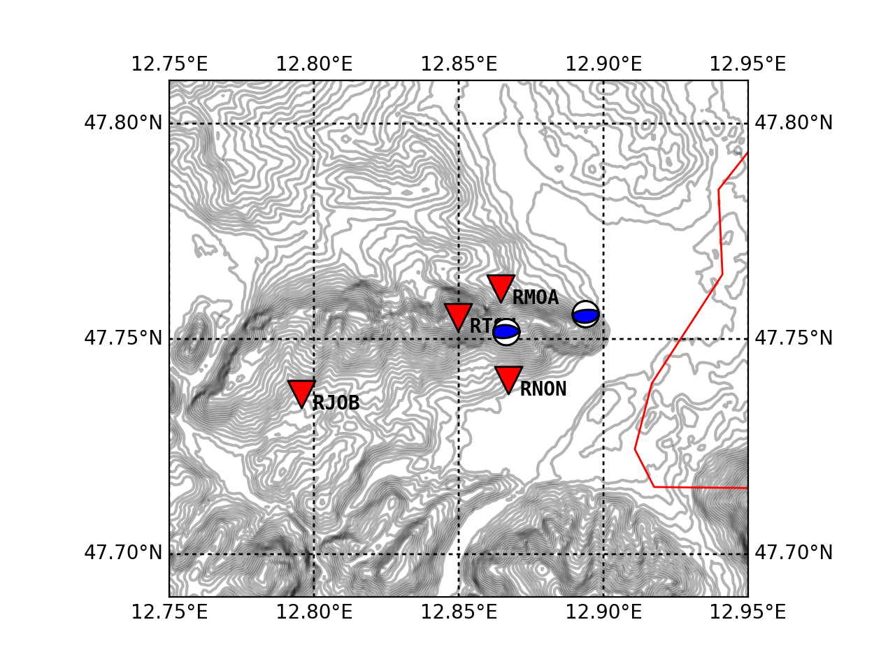
20.2. Basemap Plot of a Local Area with Beachballs
The following example shows how to plot beachballs into a basemap plot together with some stations. The example requires the basemap package (download site) to be installed. The SRTM file used can be downloaded here. The first lines of our SRTM data file (from CGIAR) look like this:
ncols         400
nrows         200
xllcorner     12°40'E
yllcorner     47°40'N
xurcorner     13°00'E
yurcorner     47°50'N
cellsize      0.00083333333333333
NODATA_value  -9999
682 681 685 690 691 689 678 670 675 680 681 679 675 671 674 680 679 679 675 671 668 664 659 660 656 655 662 666 660 659 659 658 ....
import gzip

import numpy as np
import matplotlib.pyplot as plt
from mpl_toolkits.basemap import Basemap

from obspy.imaging.beachball import beach


# read in topo data (on a regular lat/lon grid)
# (SRTM data from: http://srtm.csi.cgiar.org/)
with gzip.open("srtm_1240-1300E_4740-4750N.asc.gz") as fp:
    srtm = np.loadtxt(fp, skiprows=8)

# origin of data grid as stated in SRTM data file header
# create arrays with all lon/lat values from min to max and
lats = np.linspace(47.8333, 47.6666, srtm.shape[0])
lons = np.linspace(12.6666, 13.0000, srtm.shape[1])

# create Basemap instance with Mercator projection
# we want a slightly smaller region than covered by our SRTM data
m = Basemap(projection='merc', lon_0=13, lat_0=48, resolution="h",
            llcrnrlon=12.75, llcrnrlat=47.69, urcrnrlon=12.95, urcrnrlat=47.81)

# create grids and compute map projection coordinates for lon/lat grid
x, y = m(*np.meshgrid(lons, lats))

# Make contour plot
cs = m.contour(x, y, srtm, 40, colors="k", lw=0.5, alpha=0.3)
m.drawcountries(color="red", linewidth=1)

# Draw a lon/lat grid (20 lines for an interval of one degree)
m.drawparallels(np.linspace(47, 48, 21), labels=[1, 1, 0, 0], fmt="%.2f",
                dashes=[2, 2])
m.drawmeridians(np.linspace(12, 13, 21), labels=[0, 0, 1, 1], fmt="%.2f",
                dashes=[2, 2])

# Plot station positions and names into the map
# again we have to compute the projection of our lon/lat values
lats = [47.761659, 47.7405, 47.755100, 47.737167]
lons = [12.864466, 12.8671, 12.849660, 12.795714]
names = [" RMOA", " RNON", " RTSH", " RJOB"]
x, y = m(lons, lats)
m.scatter(x, y, 200, color="r", marker="v", edgecolor="k", zorder=3)
for i in range(len(names)):
    plt.text(x[i], y[i], names[i], va="top", family="monospace", weight="bold")

# Add beachballs for two events
lats = [47.751602, 47.75577]
lons = [12.866492, 12.893850]
x, y = m(lons, lats)
# Two focal mechanisms for beachball routine, specified as [strike, dip, rake]
focmecs = [[80, 50, 80], [85, 30, 90]]
ax = plt.gca()
for i in range(len(focmecs)):
    b = beach(focmecs[i], xy=(x[i], y[i]), width=1000, linewidth=1)
    b.set_zorder(10)
    ax.add_collection(b)

plt.show()
(Source code, png, hires.png)

Some notes:
The Python package GDAL allows you to directly read a GeoTiff into NumPy ndarray
>>> geo = gdal.Open("file.geotiff")
>>> x = geo.ReadAsArray()
GeoTiff elevation data is available e.g. from ASTER
Shading/Illumination can be added. See the basemap example plotmap_shaded.py for more info.
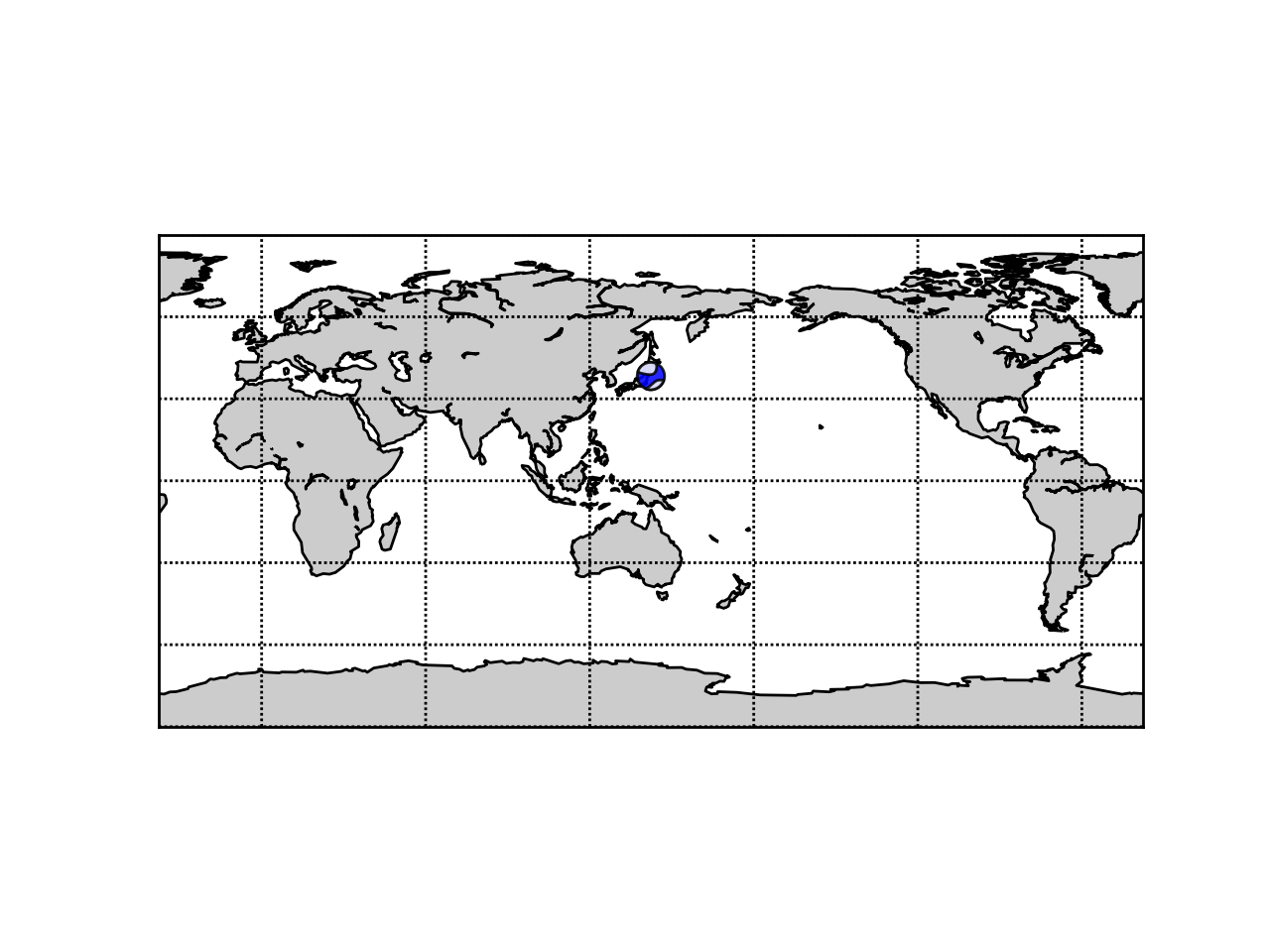
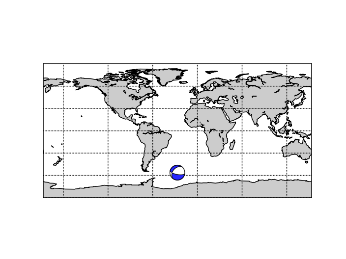
20.3. Basemap Plot of the Globe with Beachballs
import numpy as np
import matplotlib.pyplot as plt
from mpl_toolkits.basemap import Basemap

from obspy.imaging.beachball import beach


m = Basemap(projection='cyl', lon_0=142.36929, lat_0=38.3215,
            resolution='c')

m.drawcoastlines()
m.fillcontinents()
m.drawparallels(np.arange(-90., 120., 30.))
m.drawmeridians(np.arange(0., 420., 60.))
m.drawmapboundary()

x, y = m(142.36929, 38.3215)
focmecs = [0.136, -0.591, 0.455, -0.396, 0.046, -0.615]

ax = plt.gca()
b = beach(focmecs, xy=(x, y), width=10, linewidth=1, alpha=0.85)
b.set_zorder(10)
ax.add_collection(b)
plt.show()
(Source code, png, hires.png)

20.4. Basemap Plot of the Globe with Beachball using read_events
import numpy as np
import matplotlib.pyplot as plt
from mpl_toolkits.basemap import Basemap

from obspy import read_events
from obspy.imaging.beachball import beach


event = read_events(
    'https://earthquake.usgs.gov/archive/product/moment-tensor/'
    'us_20005ysu_mww/us/1470868224040/quakeml.xml', format='QUAKEML')[0]
origin = event.preferred_origin() or event.origins[0]
focmec = event.preferred_focal_mechanism() or event.focal_mechanisms[0]
tensor = focmec.moment_tensor.tensor
moment_list = [tensor.m_rr, tensor.m_tt, tensor.m_pp,
               tensor.m_rt, tensor.m_rp, tensor.m_tp]

m = Basemap(projection='cyl', lon_0=origin.longitude, lat_0=origin.latitude,
            resolution='c')

m.drawcoastlines()
m.fillcontinents()
m.drawparallels(np.arange(-90., 120., 30.))
m.drawmeridians(np.arange(0., 420., 60.))
m.drawmapboundary()

x, y = m(origin.longitude, origin.latitude)

ax = plt.gca()
b = beach(moment_list, xy=(x, y), width=20, linewidth=1, alpha=0.85)
b.set_zorder(10)
ax.add_collection(b)
plt.show()
(Source code, png, hires.png)
