13. Poles and Zeros, Frequency Response
Note
For metadata read using read_inventory() into Inventory objects (and the corresponding sub-objects Network, Station, Channel, Response), there is a convenience method to show Bode plots, see e.g. Inventory.plot_response() or Response.plot()).
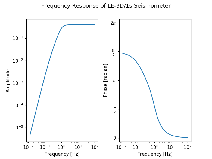
The following lines show how to calculate and visualize the frequency response of a LE-3D/1s seismometer with sampling interval 0.005s and 16384 points of fft. We want the phase to go from 0 to 2*pi, instead of the output from angle that goes from -pi to pi .
import numpy as np
import matplotlib.pyplot as plt

from obspy.signal.invsim import paz_to_freq_resp


poles = [-4.440 + 4.440j, -4.440 - 4.440j, -1.083 + 0.0j]
zeros = [0.0 + 0.0j, 0.0 + 0.0j, 0.0 + 0.0j]
scale_fac = 0.4

h, f = paz_to_freq_resp(poles, zeros, scale_fac, 0.005, 16384, freq=True)

plt.figure()
plt.subplot(121)
plt.loglog(f, abs(h))
plt.xlabel('Frequency [Hz]')
plt.ylabel('Amplitude')

plt.subplot(122)
phase = 2 * np.pi + np.unwrap(np.angle(h))
plt.semilogx(f, phase)
plt.xlabel('Frequency [Hz]')
plt.ylabel('Phase [radian]')
# ticks and tick labels at multiples of pi
plt.yticks(
    [0, np.pi / 2, np.pi, 3 * np.pi / 2, 2 * np.pi],
    ['$0$', r'$\frac{\pi}{2}$', r'$\pi$', r'$\frac{3\pi}{2}$', r'$2\pi$'])
plt.ylim(-0.2, 2 * np.pi + 0.2)
# title, centered above both subplots
plt.suptitle('Frequency Response of LE-3D/1s Seismometer')
# make more room in between subplots for the ylabel of right plot
plt.subplots_adjust(wspace=0.3)
plt.show()
(Source code, png, hires.png)
