14. Seismometer Correction/Simulation
14.1. Calculating response from filter stages using evalresp..
14.1.1. ..using a StationXML file or in general an Inventory object
When using the FDSN client the response can directly be attached to the waveforms and then subsequently removed using Stream.remove_response():
from obspy import UTCDateTime
from obspy.clients.fdsn import Client

t1 = UTCDateTime("2010-09-3T16:30:00.000")
t2 = UTCDateTime("2010-09-3T17:00:00.000")
fdsn_client = Client('IRIS')
# Fetch waveform from IRIS FDSN web service into a ObsPy stream object
# and automatically attach correct response
st = fdsn_client.get_waveforms(network='NZ', station='BFZ', location='10',
                               channel='HHZ', starttime=t1, endtime=t2,
                               attach_response=True)
# define a filter band to prevent amplifying noise during the deconvolution
pre_filt = (0.005, 0.006, 30.0, 35.0)
st.remove_response(output='DISP', pre_filt=pre_filt)
Alternatively an Inventory object can be directly passed to the Stream.remove_response(): method:
from obspy import read, read_inventory

# simply use the included example waveform
st = read()
# the corresponding response is included in ObsPy as a StationXML file
inv = read_inventory()
# the routine automatically picks the correct response for each trace
# define a filter band to prevent amplifying noise during the deconvolution
pre_filt = (0.005, 0.006, 30.0, 35.0)
st.remove_response(inventory=inv, output='DISP', pre_filt=pre_filt)
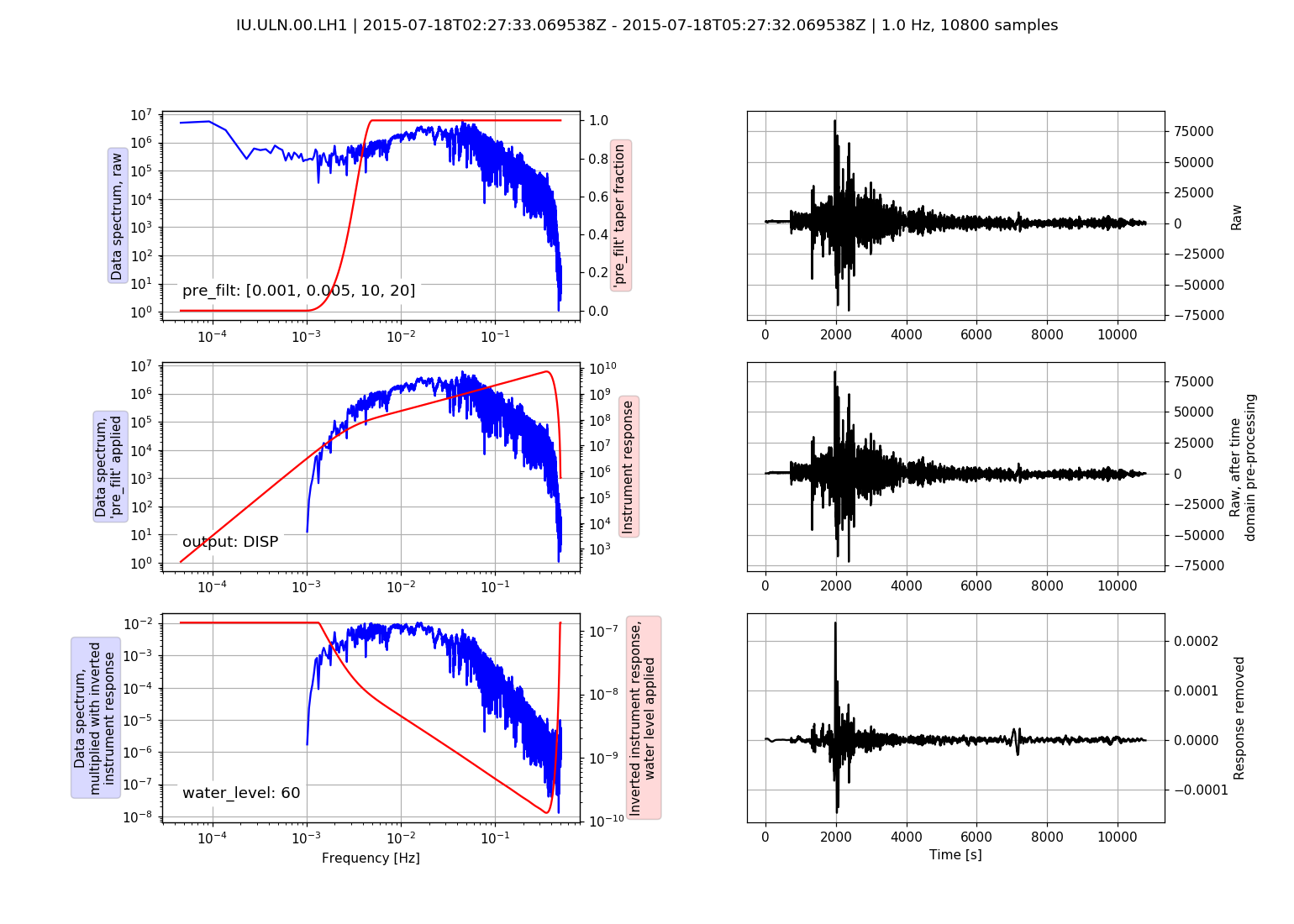
Using the plot option it is possible to visualize the individual steps during response removal in the frequency domain to check the chosen pre_filt and water_level options to stabilize the deconvolution of the inverted instrument response spectrum:
from obspy import read, read_inventory

st = read("/path/to/IU_ULN_00_LH1_2015-07-18T02.mseed")
tr = st[0]
inv = read_inventory("/path/to/IU_ULN_00_LH1.xml")
pre_filt = [0.001, 0.005, 10, 20]
tr.remove_response(inventory=inv, pre_filt=pre_filt, output="DISP",
                   water_level=60, plot=True)
(Source code, png, hires.png)

14.1.2. ..using a RESP file
It is further possible to use evalresp to evaluate the instrument response information from a RESP file.
import matplotlib.pyplot as plt
import obspy
from obspy.core.util import NamedTemporaryFile
from obspy.clients.fdsn import Client as FDSN_Client
from obspy.clients.iris import Client as OldIris_Client
# MW 7.1 Darfield earthquake, New Zealand
t1 = obspy.UTCDateTime("2010-09-3T16:30:00.000")
t2 = obspy.UTCDateTime("2010-09-3T17:00:00.000")
# Fetch waveform from IRIS FDSN web service into a ObsPy stream object
fdsn_client = FDSN_Client("IRIS")
st = fdsn_client.get_waveforms('NZ', 'BFZ', '10', 'HHZ', t1, t2)
# Download and save instrument response file into a temporary file
with NamedTemporaryFile() as tf:
respf = tf.name
old_iris_client = OldIris_Client()
# fetch RESP information from "old" IRIS web service, see obspy.fdsn
# for accessing the new IRIS FDSN web services
old_iris_client.resp('NZ', 'BFZ', '10', 'HHZ', t1, t2, filename=respf)
# make a copy to keep our original data
st_orig = st.copy()
# define a filter band to prevent amplifying noise during the deconvolution
pre_filt = (0.005, 0.006, 30.0, 35.0)
# this can be the date of your raw data or any date for which the
# SEED RESP-file is valid
date = t1
seedresp = {'filename': respf, # RESP filename
# when using Trace/Stream.simulate() the "date" parameter can
# also be omitted, and the starttime of the trace is then used.
'date': date,
# Units to return response in ('DIS', 'VEL' or ACC)
'units': 'DIS'
}
# Remove instrument response using the information from the given RESP file
st.simulate(paz_remove=None, pre_filt=pre_filt, seedresp=seedresp)
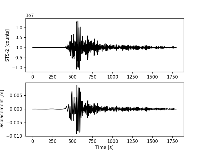
# plot original and simulated data
tr = st[0]
tr_orig = st_orig[0]
time = tr.times()
plt.subplot(211)
plt.plot(time, tr_orig.data, 'k')
plt.ylabel('STS-2 [counts]')
plt.subplot(212)
plt.plot(time, tr.data, 'k')
plt.ylabel('Displacement [m]')
plt.xlabel('Time [s]')
plt.show()
(Source code, png, hires.png)

14.1.3. ..using a Dataless/Full SEED file (or XMLSEED file)
A Parser object created using a Dataless SEED file can also be used. For each trace the respective RESP response data is extracted internally then. When using Stream/Trace‘s simulate() convenience methods the “date” parameter can be omitted (each trace’s start time is used internally).
import obspy
from obspy.io.xseed import Parser


st = obspy.read("https://examples.obspy.org/BW.BGLD..EH.D.2010.037")
parser = Parser("https://examples.obspy.org/dataless.seed.BW_BGLD")
st.simulate(seedresp={'filename': parser, 'units': "DIS"})
14.2. Using a PAZ dictionary
The following script shows how to simulate a 1Hz seismometer from a STS-2 seismometer with the given poles and zeros. Poles, zeros, gain (A0 normalization factor) and sensitivity (overall sensitivity) are specified as keys of a dictionary.
import obspy
from obspy.signal.invsim import corn_freq_2_paz
paz_sts2 = {
'poles': [-0.037004 + 0.037016j, -0.037004 - 0.037016j, -251.33 + 0j,
- 131.04 - 467.29j, -131.04 + 467.29j],
'zeros': [0j, 0j],
'gain': 60077000.0,
'sensitivity': 2516778400.0}
paz_1hz = corn_freq_2_paz(1.0, damp=0.707) # 1Hz instrument
paz_1hz['sensitivity'] = 1.0
st = obspy.read()
# make a copy to keep our original data
st_orig = st.copy()
# Simulate instrument given poles, zeros and gain of
# the original and desired instrument
st.simulate(paz_remove=paz_sts2, paz_simulate=paz_1hz)
# plot original and simulated data
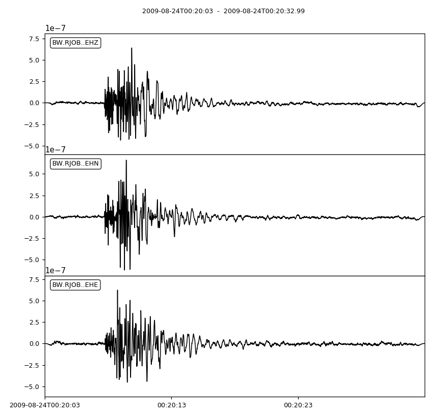
st_orig.plot()
st.plot()
(Source code, png, hires.png)
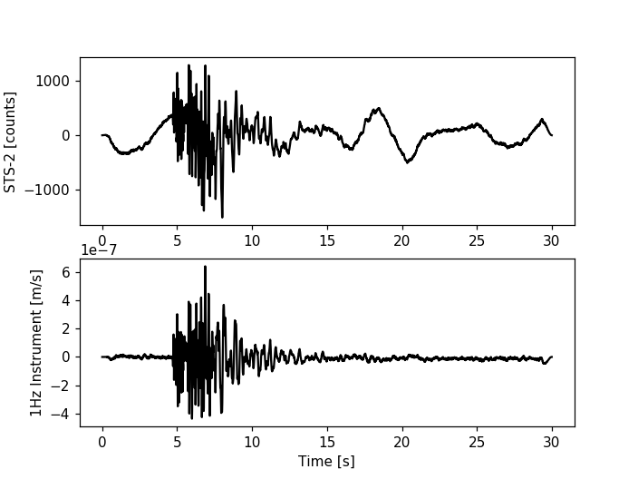
For more customized plotting we could also work with matplotlib manually from here:
import numpy as np
import matplotlib.pyplot as plt

tr = st[0]
tr_orig = st_orig[0]

t = np.arange(tr.stats.npts) / tr.stats.sampling_rate

plt.subplot(211)
plt.plot(t, tr_orig.data, 'k')
plt.ylabel('STS-2 [counts]')
plt.subplot(212)
plt.plot(t, tr.data, 'k')
plt.ylabel('1Hz Instrument [m/s]')
plt.xlabel('Time [s]')
plt.show()
(Source code, png, hires.png)