Cross-Correlation Detector
These code snippets show how to use the function
correlation_detector().
Detection based on one component
In the first example we will determine the origin time of the 2017 North Korean nuclear test, by using a template of another test in 2013. We will use only a single channel of the station IC.MDJ.
from obspy import read, UTCDateTime as UTC
from obspy.signal.cross_correlation import correlation_detector

template = read('https://examples.obspy.org/IC.MDJ.2013.043.mseed')
template.filter('bandpass', freqmin=0.5, freqmax=2)
template.plot()
(Source code, png)

pick = UTC('2013-02-12T02:58:44.95')
template.trim(pick, pick + 150)

stream = read('https://examples.obspy.org/IC.MDJ.2017.246.mseed')
stream.filter('bandpass', freqmin=0.5, freqmax=2)
height = 0.3  # similarity threshold
distance = 10  # distance between detections in seconds
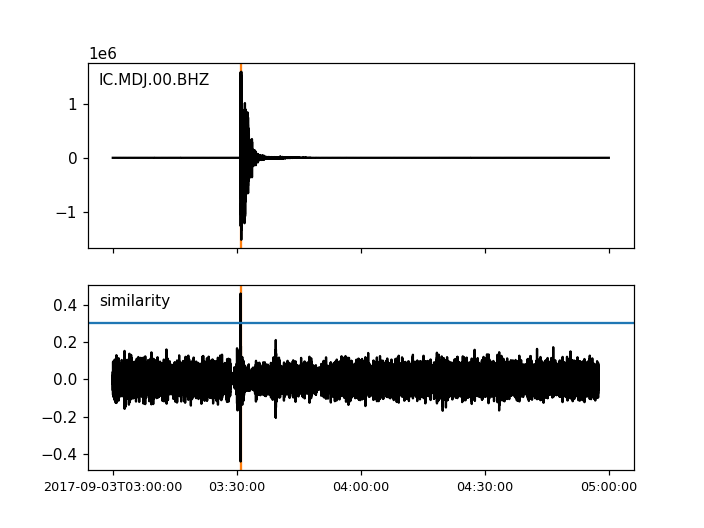
detections, sims = correlation_detector(stream, template, height, distance, plot=stream)
(Source code, png)

The above detection corresponds to the start time of the template. If the template of the 2013 explosion is associated with its origin time, the origin time of the 2017 explosion can be directly determined. The threshold is lowered to 0.2 to detect also the collapse which occurred around 8 minutes after the 2013 test.
utc_nuclear_test_2013 = UTC('2013-02-12T02:57:51')
height = 0.2  # lower threshold
detections, sims = correlation_detector(
        stream, template, height, distance, template_times=utc_nuclear_test_2013)
detections
[{'time': 2017-09-03T03:30:01.371731Z,
  'similarity': 0.46020218652131695,
  'template_id': 0},
 {'time': 2017-09-03T03:38:31.821731Z,
  'similarity': 0.21099726068286417,
  'template_id': 0}]
Multi-station detection of swarm earthquakes with multiple templates
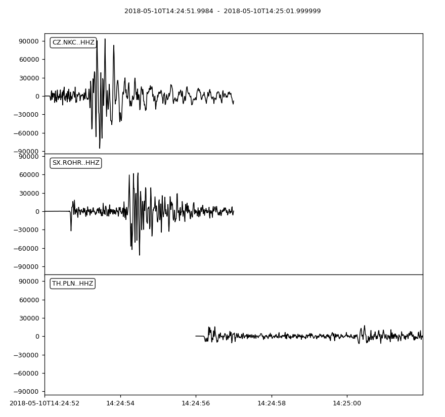
In this example we load 12 hours of data from the start of the 2018 Novy Kostel earthquake swarm in Northwestern Bohemia/Czech Republic near the border to Germany. The example stream consists only of Z component data. Data are filtered by a highpass. Origin times and magnitudes of the two larger earthquakes in this period are extracted from the WEBNET earthquake catalog. The template waveforms of these earthquakes are selected and one template is plotted. After that, cross-correlations are calculated and other, similar earthquakes in the swarm are detected.
from obspy import read, Trace, UTCDateTime as UTC
from obspy.signal.cross_correlation import correlation_detector

stream = read('https://examples.obspy.org/NKC_PLN_ROHR.HHZ.2018.130.mseed')
stream.filter('highpass', freq=1, zerophase=True)

otimes = [UTC('2018-05-10 14:24:50'), UTC('2018-05-10 19:42:08')]
templates = []
for otime in otimes:
    template = stream.select(station='NKC').slice(otime + 2, otime + 7)
    template += stream.select(station='ROHR').slice(otime + 2, otime + 7)
    template += stream.select(station='PLN').slice(otime + 6, otime + 12)
    templates.append(template)

template_magnitudes = [2.9, 2.8]
template_names = ['1st template', '2nd template']
templates[0].plot()
(Source code, png)

height = 0.5  # similarity threshold
distance = 10  # distance between detections in seconds
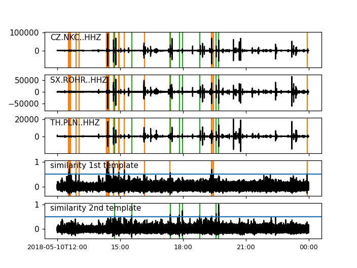
detections, sims = correlation_detector(stream, templates, height, distance, template_names=template_names, plot=stream)
(Source code, png)

By default, the similarity is calculated by the mean of cross-correlations. In the following, we create a custom function which calculates the similarity trace from a stream of cross-correlations and applies the constraint that the cross-correlation should be larger than 0.5 at all stations. The function is then passed to the detector.
def similarity_component_thres(ccs, thres, num_components):
    """Return Trace with mean of ccs
    and set values to zero if number of components above threshold is not reached"""
    ccmatrix = np.array([tr.data for tr in ccs])
    header = dict(sampling_rate=ccs[0].stats.sampling_rate,
                  starttime=ccs[0].stats.starttime)
    comp_thres = np.sum(ccmatrix > thres, axis=0) >= num_components
    data = np.mean(ccmatrix, axis=0) * comp_thres
    return Trace(data=data, header=header)

def simf(ccs):
    return similarity_component_thres(ccs, 0.5, 3)

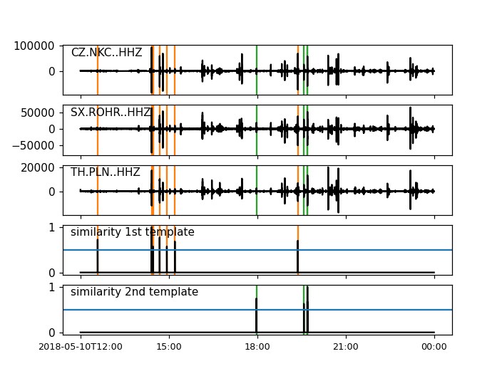
detections, sims = correlation_detector(
        stream, templates, height, distance, similarity_func=simf, plot=stream,
        template_times=otimes, template_magnitudes=template_magnitudes, template_names=template_names)
(Source code, png)

Now, we have only 11 detections, probably from two specific earthquake clusters. To get more detections, we need to relax the constraints again. Another possibility is to calculate the envelope of the data before applying the correlation or to mute the coda waves in the template by setting corresponding data values to zero.
We passed the magnitudes of the templates to the detector. Therefore, the detections include magnitudes estimated from the amplitude ratios between data and templates:
detections
[{'time': 2018-05-10T12:34:56.631599Z,
  'similarity': 0.72489172487200071,
  'template_name': '1st template',
  'template_id': 0,
  'amplitude_ratio': 0.042826872986209588,
  'magnitude': 1.0756218205928332},
 {'time': 2018-05-10T14:24:50.001599Z,
  'similarity': 1.0000000000000027,
  'template_name': '1st template',
  'template_id': 0,
  'amplitude_ratio': 1.0,
  'magnitude': 2.8999999999999999},
 {'time': 2018-05-10T14:27:50.921599Z,
  'similarity': 0.57155043392492588,
  'template_name': '1st template',
  'template_id': 0,
  'amplitude_ratio': 0.019130460518598909,
  'magnitude': 0.60896723296053024},
 {'time': 2018-05-10T14:41:07.691599Z,
  'similarity': 0.772879074393792,
  'template_name': '1st template',
  'template_id': 0,
  'amplitude_ratio': 0.57507924545222067,
  'magnitude': 2.5796369256528813},
 {'time': 2018-05-10T14:55:50.001599Z,
  'similarity': 0.57467717600499058,
  'template_name': '1st template',
  'template_id': 0,
  'amplitude_ratio': 0.078631249252299668,
  'magnitude': 1.4274602340872211},
 {'time': 2018-05-10T15:12:10.141599Z,
  'similarity': 0.6852082687836063,
  'template_name': '1st template',
  'template_id': 0,
  'amplitude_ratio': 0.11301513001944399,
  'magnitude': 1.6375154520085005},
 {'time': 2018-05-10T17:58:11.861599Z,
  'similarity': 0.74731725616064482,
  'template_name': '2nd template',
  'template_id': 1,
  'amplitude_ratio': 0.23222879133919266,
  'magnitude': 1.9545547491304716},
 {'time': 2018-05-10T19:22:29.511599Z,
  'similarity': 0.70112087830579739,
  'template_name': '1st template',
  'template_id': 0,
  'amplitude_ratio': 0.68929540439903225,
  'magnitude': 2.6845405106924867},
 {'time': 2018-05-10T19:34:50.271599Z,
  'similarity': 0.63060024934168146,
  'template_name': '2nd template',
  'template_id': 1,
  'amplitude_ratio': 0.51910269908035278,
  'magnitude': 2.4203377160050512},
 {'time': 2018-05-10T19:41:55.021599Z,
  'similarity': 0.68000312618108072,
  'template_name': '2nd template',
  'template_id': 1,
  'amplitude_ratio': 0.054704354180392788,
  'magnitude': 1.1173625270371177},
 {'time': 2018-05-10T19:42:08.001599Z,
  'similarity': 0.99999999999999434,
  'template_name': '2nd template',
  'template_id': 1,
  'amplitude_ratio': 1.0,
  'magnitude': 2.7999999999999998}]