Module for handling station metadata
This module provides a class hierarchy to consistently handle station metadata. This class hierarchy is closely modelled after the upcoming de-facto standard format FDSN StationXML which was developed as a human readable XML replacement for Dataless SEED.
Note
EarthScope/IRIS is maintaining a Java tool for converting dataless SEED into StationXML and vice versa at https://seiscode.iris.washington.edu/projects/stationxml-converter
- copyright:
The ObsPy Development Team (devs@obspy.org) & Chad Trabant
- license:
GNU Lesser General Public License, Version 3 (https://www.gnu.org/copyleft/lesser.html)
Reading
StationXML files can be read using the
read_inventory() function that
returns an Inventory object.
>>> from obspy import read_inventory
>>> inv = read_inventory("/path/to/BW_RJOB.xml")
>>> inv
<obspy.core.inventory.inventory.Inventory object at 0x...>
>>> print(inv)
Inventory created at 2013-12-07T18:00:42.878000Z
    Created by: fdsn-stationxml-converter/1.0.0
            http://www.iris.edu/fdsnstationconverter
    Sending institution: Erdbebendienst Bayern
    Contains:
        Networks (1):
            BW
        Stations (1):
            BW.RJOB (Jochberg, Bavaria, BW-Net)
        Channels (3):
            BW.RJOB..EHZ, BW.RJOB..EHN, BW.RJOB..EHE
The file format in principle is autodetected. However, the autodetection uses the official StationXML XSD schema and unfortunately many real world files currently show minor deviations from the official StationXML definition causing the autodetection to fail. Thus, manually specifying the format is a good idea:
>>> inv = read_inventory("/path/to/BW_RJOB.xml", format="STATIONXML")
Class hierarchy
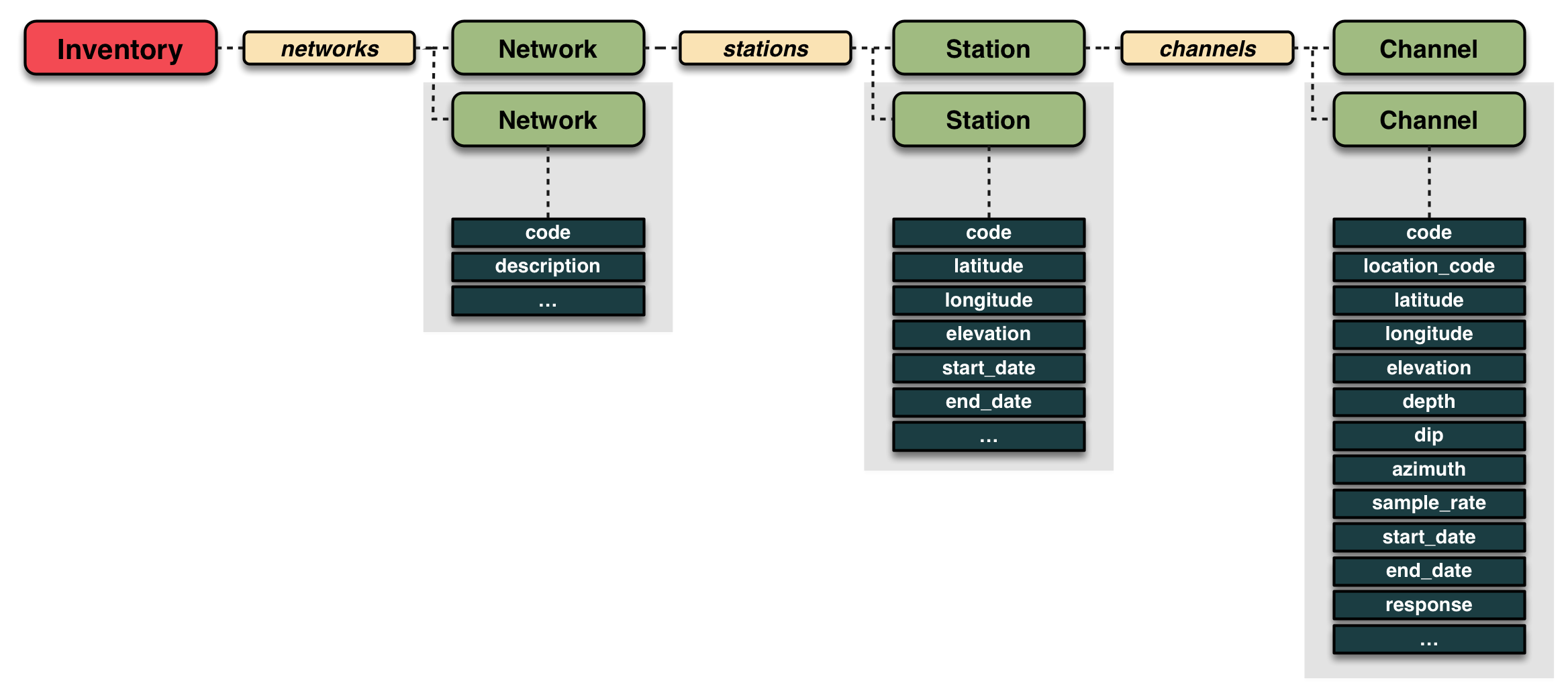
The Inventory class has a hierarchical
structure, starting with a list of Networks, each containing a list of
Stations which again each
contain a list of Channels.
The Responses are
attached to the channels as an attribute.
>>> net = inv[0]
>>> net
<obspy.core.inventory.network.Network object at 0x...>
>>> print(net)
Network BW (BayernNetz)
    Station Count: None/None (Selected/Total)
    -- - --
    Access: UNKNOWN
    Contains:
        Stations (1):
            BW.RJOB (Jochberg, Bavaria, BW-Net)
        Channels (3):
            BW.RJOB..EHZ, BW.RJOB..EHN, BW.RJOB..EHE
>>> sta = net[0]
>>> print(sta)
Station RJOB (Jochberg, Bavaria, BW-Net)
    Station Code: RJOB
    Channel Count: None/None (Selected/Total)
    2007-12-17T00:00:00.000000Z -
    Access: None
    Latitude: 47.7372, Longitude: 12.7957, Elevation: 860.0 m
    Available Channels:
        ..EH[ZNE]   200.0 Hz  2007-12-17(351) -
>>> cha = sta[0]
>>> print(cha)
Channel 'EHZ', Location ''
    Time range: 2007-12-17T00:00:00.000000Z - --
    Latitude: 47.7372, Longitude: 12.7957, Elevation: 860.0 m, Local Depth: 0.0 m
    Azimuth: 0.00 degrees from north, clockwise
    Dip: -90.00 degrees down from horizontal
    Channel types: TRIGGERED, GEOPHYSICAL
    Sampling Rate: 200.00 Hz
    Sensor (Description): Streckeisen STS-2/N seismometer (None)
    Response information available
>>> print(cha.response)
Channel Response
   From M/S (Velocity in Meters Per Second) to COUNTS (Digital Counts)
   Overall Sensitivity: 2.5168e+09 defined at 0.020 Hz
   4 stages:
      Stage 1: PolesZerosResponseStage from M/S to V, gain: 1500
      Stage 2: CoefficientsTypeResponseStage from V to COUNTS, gain: 1.67...
      Stage 3: FIRResponseStage from COUNTS to COUNTS, gain: 1
      Stage 4: FIRResponseStage from COUNTS to COUNTS, gain: 1
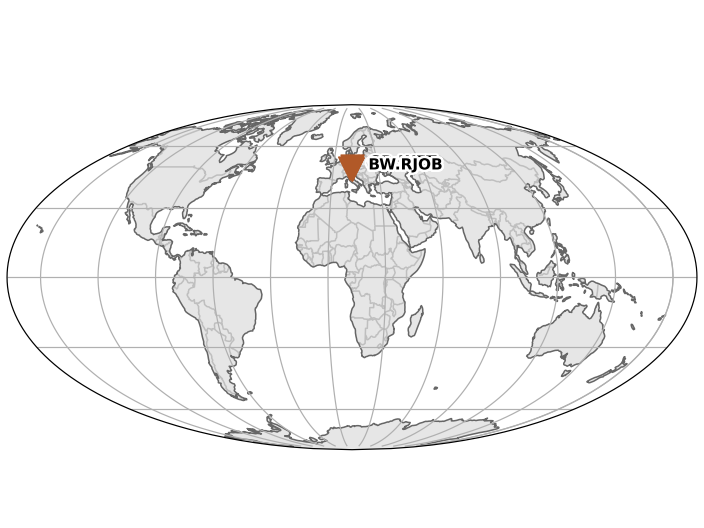
Preview plots of station map and instrument response
For station metadata, preview plot routines for geographic location of stations as well as bode plots for channel instrument response information are available. The routines for station map plots are:
For example:
>>> from obspy import read_inventory
>>> inv = read_inventory()
>>> inv.plot()
(Source code, png)

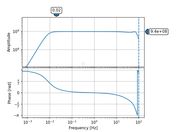
The routines for bode plots of channel instrument response are:
For example:
>>> from obspy import read_inventory
>>> inv = read_inventory()
>>> resp = inv[0][0][0].response
>>> resp.plot(0.001, output="VEL")
(Source code, png)
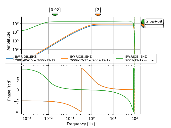
When plotting stations with instrumentation changes, epoch times can be added to the legend labels:
>>> from obspy import read_inventory
>>> inv = read_inventory()
>>> inv = inv.select(station='RJOB', channel='EHZ')
>>> inv.plot_response(0.001, label_epoch_dates=True)
(Source code, png)
For more examples see the Obspy Gallery.
Dealing with the Response information
The get_evalresp_response()
method will call some functions within evalresp to generate the response.
>>> response = cha.response
>>> response, freqs = response.get_evalresp_response(0.1, 16384, output="VEL")
>>> print(response)
 [  0.00000000e+00 +0.00000000e+00j  -1.36383361e+07 +1.42086194e+06j
   -5.36470300e+07 +1.13620679e+07j ...,   2.48907496e+09 -3.94151237e+08j
    2.48906963e+09 -3.94200472e+08j   2.48906430e+09 -3.94249707e+08j]
Some convenience methods to perform an instrument correction on
Stream (and Trace)
objects are available and most users will want to use those. The
remove_response() method deconvolves the
instrument response in-place. As always see the corresponding docs pages for a
full list of options and a more detailed explanation.
>>> from obspy import read
>>> st = read()
>>> inv = read_inventory("/path/to/BW_RJOB.xml")
>>> st.remove_response(
...     inventory=inv, output="VEL", water_level=20)
<obspy.core.stream.Stream object at 0x...>
Writing
Inventory objects can be exported to
StationXML files, e.g. after making modifications.
>>> inv.write('my_inventory.xml', format='STATIONXML')
Classes & Functions
Function to read inventory files. |
Modules
Provides the Inventory class. |
|
Provides the Network class. |
|
Provides the Station class. |
|
Provides the Channel class. |
|
Classes related to instrument responses. |
|
Utility objects. |