Travel Time and Ray Path Plotting
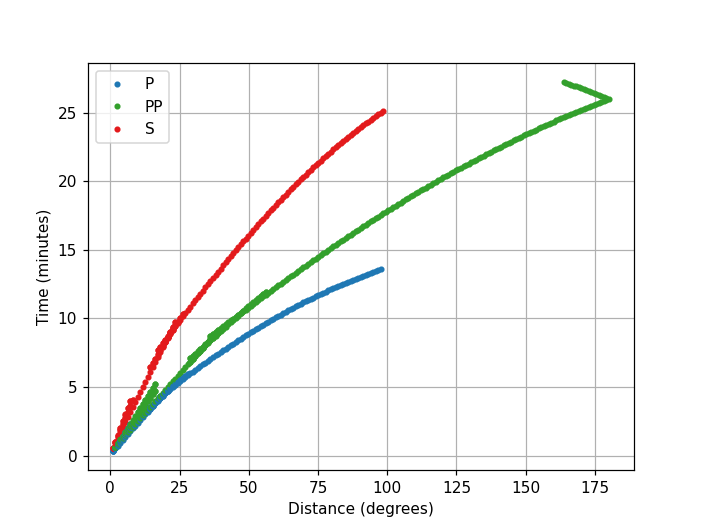
Travel Time Plot
The following lines show how to use the convenience wrapper function
plot_travel_times() to plot the travel times for a
given distance range and selected phases, calculated with the
iasp91 velocity model.
from obspy.taup import plot_travel_times
import matplotlib.pyplot as plt

fig, ax = plt.subplots()
ax = plot_travel_times(source_depth=10, ax=ax, fig=fig,
                       phase_list=['P', 'PP', 'S'], npoints=200)
(Source code, png)
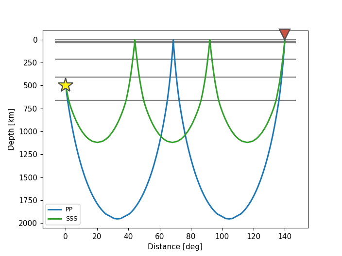
Cartesian Ray Paths
The following lines show how to plot the ray paths for a given
distance, and phase(s). The ray paths are calculated with the iasp91
velocity model, and plotted on a Cartesian map, using the
plot_rays() method of the class
obspy.taup.tau.Arrivals.
from obspy.taup import TauPyModel

model = TauPyModel(model='iasp91')
arrivals = model.get_ray_paths(500, 140, phase_list=['PP', 'SSS'])
arrivals.plot_rays(plot_type='cartesian', phase_list=['PP', 'SSS'],
                   plot_all=False, legend=True)
(Source code, png)
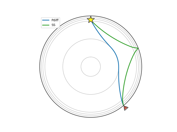
Spherical Ray Paths
The following lines show how to plot the ray paths for a given
distance, and phase(s). The ray paths are calculated with the
iasp91 velocity model, and plotted on a spherical map, using the
plot_rays() method of the class
obspy.taup.tau.Arrivals.
from obspy.taup import TauPyModel

model = TauPyModel(model='iasp91')
arrivals = model.get_ray_paths(500, 140, phase_list=['Pdiff', 'SS'])
arrivals.plot_rays(plot_type='spherical', phase_list=['Pdiff', 'SS'],
                   legend=True)
(Source code, png)
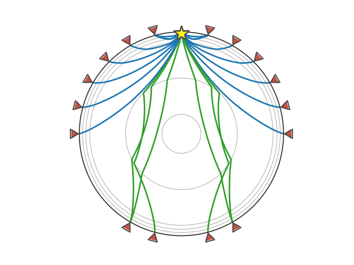
Ray Paths for Multiple Distances
The following lines plot the ray paths for several epicentral
distances, and phases. The rays are calculated with the iasp91
velocity model, and the plot is made using the convenience wrapper
function plot_ray_paths().
from obspy.taup.tau import plot_ray_paths
import matplotlib.pyplot as plt

fig, ax = plt.subplots(subplot_kw=dict(polar=True))
ax = plot_ray_paths(source_depth=100, ax=ax, fig=fig, phase_list=['P', 'PKP'],
                    npoints=25)
(Source code, png)
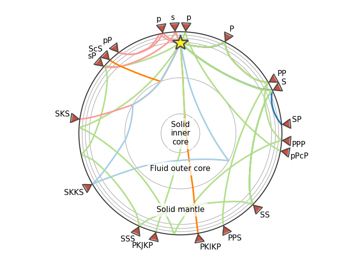
For examples with rays for a single epicentral distance, try the
plot_rays() method in the previous
section. The following is a more advanced example with a custom list of phases
and distances:
import numpy as np
import matplotlib.pyplot as plt

from obspy.taup import TauPyModel


PHASES = [
    # Phase, distance
    ('P', 26),
    ('PP', 60),
    ('PPP', 94),
    ('PPS', 155),
    ('p', 3),
    ('pPcP', 100),
    ('PKIKP', 170),
    ('PKJKP', 194),
    ('S', 65),
    ('SP', 85),
    ('SS', 134.5),
    ('SSS', 204),
    ('p', -10),
    ('pP', -37.5),
    ('s', -3),
    ('sP', -49),
    ('ScS', -44),
    ('SKS', -82),
    ('SKKS', -120),
]

model = TauPyModel(model='iasp91')

fig, ax = plt.subplots(subplot_kw=dict(polar=True))

# Plot all pre-determined phases
for phase, distance in PHASES:
    arrivals = model.get_ray_paths(700, distance, phase_list=[phase])
    ax = arrivals.plot_rays(plot_type='spherical',
                            legend=False, label_arrivals=True,
                            plot_all=True,
                            show=False, ax=ax)

# Annotate regions
ax.text(0, 0, 'Solid\ninner\ncore',
        horizontalalignment='center', verticalalignment='center',
        bbox=dict(facecolor='white', edgecolor='none', alpha=0.7))
ocr = (model.model.radius_of_planet -
       (model.model.s_mod.v_mod.iocb_depth +
        model.model.s_mod.v_mod.cmb_depth) / 2)
ax.text(np.deg2rad(180), ocr, 'Fluid outer core',
        horizontalalignment='center',
        bbox=dict(facecolor='white', edgecolor='none', alpha=0.7))
mr = model.model.radius_of_planet - model.model.s_mod.v_mod.cmb_depth / 2
ax.text(np.deg2rad(180), mr, 'Solid mantle',
        horizontalalignment='center',
        bbox=dict(facecolor='white', edgecolor='none', alpha=0.7))

plt.show()
(Source code, png)
