obspy.core.inventory.inventory.Inventory.plot

Inventory.plot(projection='global', resolution='l', continent_fill_color='0.9', water_fill_color='1.0', marker='v', size=225, label=True, color='#b15928', color_per_network=False, colormap='Paired', legend='upper left', time=None, show=True, outfile=None, method=None, fig=None, **kwargs)

Creates a preview map of all networks/stations in current inventory object.

Parameters:

• projection (str, optional) –

  The map projection. Currently supported are:

  • "global" (Will plot the whole world.)

  • "ortho" (Will center around the mean lat/long.)

  • "local" (Will plot around local events)

  Defaults to "global"

• resolution (str, optional) –

  Resolution of the boundary database to use. Possible values are:

  • "c" (crude)

  • "l" (low)

  • "i" (intermediate)

  • "h" (high)

  • "f" (full)

  Defaults to "l"

• continent_fill_color (valid matplotlib color, optional) – Color of the continents. Defaults to "0.9" which is a light gray.

• water_fill_color (valid matplotlib color, optional) – Color of all water bodies. Defaults to "white".

• marker (str) – Marker symbol (see matplotlib.pyplot.scatter()).

• size (float) – Marker size (see matplotlib.pyplot.scatter()).

• label (bool) – Whether to label stations with “network.station” or not.

• color (str) – Face color of marker symbol (see matplotlib.pyplot.scatter()). Defaults to the first color from the single-element “Paired” color map.

• color_per_network (bool or dict) – If set to True, each network will be drawn in a different color. A dictionary can be provided that maps network codes to color values (e.g. color_per_network={"GR": "black", "II": "green"}).

• colormap (str, valid matplotlib colormap, optional) – Only used if color_per_network=True. Specifies which colormap is used to draw the colors for the individual networks. Defaults to the “Paired” color map.

• legend (str or None) – Location string for legend, if networks are plotted in different colors (i.e. option color_per_network in use). See matplotlib.pyplot.legend() for possible values for legend location string. To disable legend set to None.

• time (UTCDateTime) – Only plot stations available at given point in time.

• show (bool) – Whether to show the figure after plotting or not. Can be used to do further customization of the plot before showing it.

• outfile (str) – Output file path to directly save the resulting image (e.g. "/tmp/image.png"). Overrides the show option, image will not be displayed interactively. The given path/file name is also used to automatically determine the output format. Supported file formats depend on your matplotlib backend. Most backends support png, pdf, ps, eps and svg. Defaults to None.

• method (str) –

  Method to use for plotting. Possible values are:

  • 'cartopy' to use the Cartopy library

  • None to use the best available library

  Defaults to None.

• fig (matplotlib.figure.Figure) – Figure instance to reuse, returned from a previous inventory/catalog plot call with method=cartopy. If a previous cartopy plot is reused, any kwargs regarding the cartopy plot setup will be ignored (i.e. projection, resolution, continent_fill_color, water_fill_color). Note that multiple plots using colorbars likely are problematic, but e.g. one station plot (without colorbar) and one event plot (with colorbar) together should work well.

Returns:

Figure instance with the plot.

Example

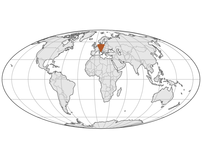
Mollweide projection for global overview:

>>> from obspy import read_inventory
>>> inv = read_inventory()
>>> inv.plot(label=False)  

(Source code, png)

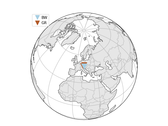
Orthographic projection, automatic colors per network:

>>> inv.plot(projection="ortho", label=False,
...          color_per_network=True)  

(Source code, png)

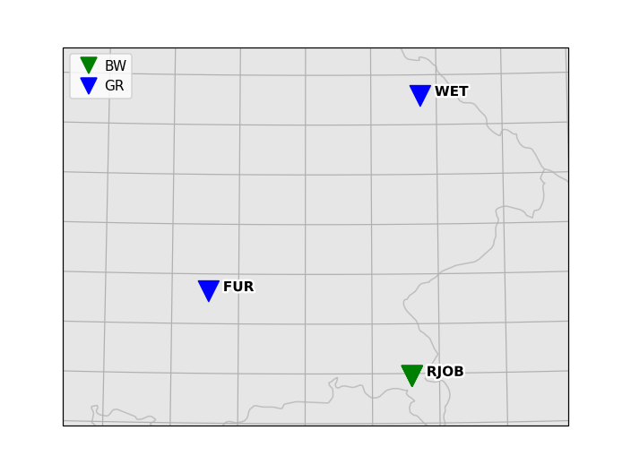
Local (Albers equal area) projection, with custom colors:

>>> colors = {'GR': 'blue', 'BW': 'green'}
>>> inv.plot(projection="local",
...          color_per_network=colors)  

(Source code, png)

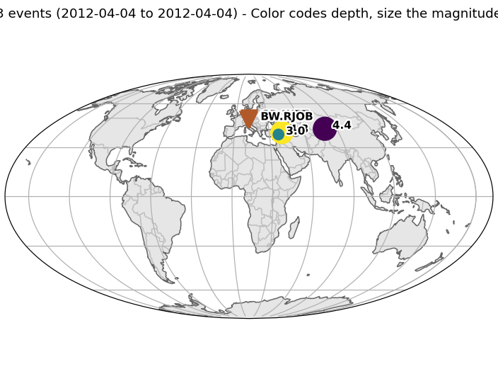
Combining a station and event plot:

>>> from obspy import read_inventory, read_events
>>> inv = read_inventory()
>>> cat = read_events()
>>> fig = inv.plot(show=False)  
>>> cat.plot(fig=fig)  

(Source code, png)