obspy.signal - Signal processing routines for ObsPy
Capabilities include filtering, triggering, rotation, instrument correction and coordinate transformations.
- copyright
The ObsPy Development Team (devs@obspy.org)
- license
GNU Lesser General Public License, Version 3 (https://www.gnu.org/copyleft/lesser.html)
Filter
The filter module provides various filters, including
different bandpass, lowpass, highpass, bandstop and FIR filter.
Warning
Before filtering you should make sure that data is demeaned/detrended, e.g.
using detrend(). Otherwise there can be
massive artifacts from filtering.
The following example shows how to highpass a seismogram at 1.0Hz. In the example only the first trace is processed to see the changes in comparison with the other traces in the plot.
Note
The filter takes the data explicitly as argument (i.e. an
numpy.ndarray) and therefore the sampling_rate needs to be
also specified. It returns the filtered data. For
Stream and Trace
objects simply use their respective filtering methods
Stream.filter() and
Trace.filter().
>>> from obspy import read
>>> import obspy.signal
>>> st = read()
>>> tr = st[0]
>>> tr.data = obspy.signal.filter.highpass(
...     tr.data, 1.0, corners=1, zerophase=True, df=tr.stats.sampling_rate)
>>> st.plot()
Working with the convenience methods implemented on
Stream/Trace
works similar:
>>> tr.filter('highpass', freq=1.0, corners=1, zerophase=True)
...
<...Trace object at 0x...>
Instrument Correction
The response of the instrument can be removed by the
invsim module. The following example shows how to remove
the the instrument response of a STS2 and simulate an instrument with 2Hz
corner frequency.
>>> from obspy import read
>>> st = read()
>>> st.plot()
Now we apply the instrument correction and simulation:
>>> from obspy.signal.invsim import simulate_seismometer, corn_freq_2_paz
>>> inst2hz = corn_freq_2_paz(2.0)
>>> sts2 = {'gain': 60077000.0,
...         'poles': [(-0.037004+0.037016j),
...                   (-0.037004-0.037016j),
...                   (-251.33+0j),
...                   (-131.04-467.29j),
...                   (-131.04+467.29j)],
...         'sensitivity': 2516778400.0,
...         'zeros': [0j, 0j]}
>>> for tr in st:
...     df = tr.stats.sampling_rate
...     tr.data = simulate_seismometer(tr.data, df, paz_remove=sts2,
...                                    paz_simulate=inst2hz,
...                                    water_level=60.0)
>>> st.plot()
Again, there are convenience methods implemented on
Stream/Trace:
>>> tr.simulate(paz_remove=sts2, paz_simulate=inst2hz, water_level=60.0)
...
<...Trace object at 0x...>
Trigger
The trigger module provides various triggering algorithms,
including different STA/LTA routines, Z-Detector, AR picker and the P-picker by
M. Bear. The implementation is based on [Withers1998] and [Baer1987].
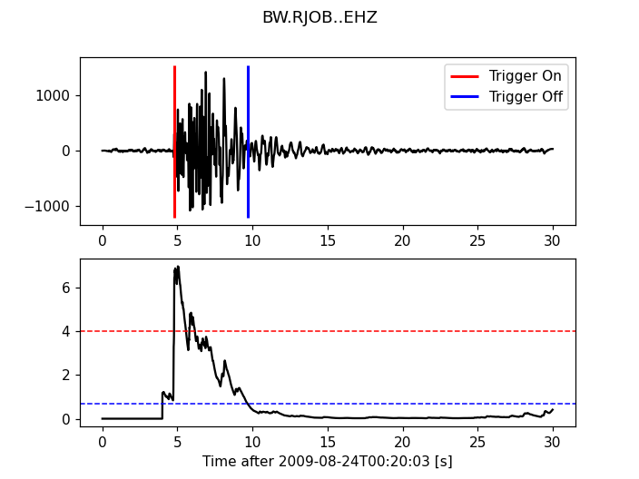
The following example demonstrates a recursive STA/LTA triggering:
>>> from obspy import read
>>> from obspy.signal.trigger import recursive_sta_lta, plot_trigger
>>> st = read()
>>> tr = st.select(component="Z")[0]
>>> tr.filter("bandpass", freqmin=1, freqmax=20)
<...Trace object at 0x...>
>>> sta = 0.5
>>> lta = 4
>>> cft = recursive_sta_lta(tr.data, int(sta * tr.stats.sampling_rate),
...                        int(lta * tr.stats.sampling_rate))
>>> thrOn = 4
>>> thrOff = 0.7
>>> plot_trigger(tr, cft, thrOn, thrOff)
(Source code, png)

There is also a convenience method implemented on
Stream/Trace.
It works on and overwrites the traces waveform data and is intended for batch
processing rather than for interactive determination of triggering parameters.
But it also means that the trace’s built-in methods can be used.
>>> tr.trigger("recstalta", sta=0.5, lta=4)
<...Trace object at 0x...>
>>> tr.plot()
For more examples check out the trigger in the Tutorial. For
network coincidence refer to obspy.signal.trigger.coincidence_trigger()
and the same page in the Tutorial. For automated use see the following
stalta example scripts.
Classes & Functions
Method for Seismic-Array-Beamforming/FK-Analysis/Capon |
|
This routine calculates the best-fitting rigid body rotation and uniform strain as functions of time, and their formal errors, given three-component ground motion time series recorded on a seismic array. |
|
Pick P and S arrivals with an AR-AIC + STA/LTA algorithm. |
|
Butterworth-Bandpass Filter. |
|
Butterworth-Bandstop Filter. |
|
Computes the carlSTAtrig characteristic function. |
|
Computes the standard STA/LTA from a given input array a. |
|
Perform a network coincidence trigger. |
|
Convert corner frequency and damping to poles and zeros. |
|
Cosine Taper. |
|
Delayed STA/LTA. |
|
Envelope of a function. |
|
Wrapper around some scipy interpolation functions. |
|
Implements the weighted average slopes interpolation scheme proposed in [Wiggins1976] for evenly sampled data. |
|
Estimate local magnitude. |
|
Get the instrument response from a SEED RESP-file. |
|
Butterworth-Highpass Filter. |
|
Butterworth-Lowpass Filter. |
|
Convert Poles and Zeros (PAZ) to frequency response. |
|
Wrapper for P-picker routine by M. |
|
Method carrying out polarization analysis with the [Flinn1965b], [Jurkevics1988], ParticleMotion, or [Vidale1986] algorithm. |
|
Use linear least squares to fit a function, f, to data. |
|
Class to compile probabilistic power spectral densities for one combination of network/station/location/channel/sampling_rate. |
|
A container for MiniSEED specific metadata, including quality control parameters. |
|
Recursive STA/LTA. |
|
Rotates horizontal components of a seismogram. |
|
Simulate/Correct seismometer. |
|
Transform lon, lat to km with reference to orig_lon and orig_lat on the elliptic Earth. |
|
Transform x, y [km] to decimal degree in reference to orig_lon and orig_lat |
|
Cross-correlation of two signals up to a specified maximal shift. |
|
Z-detector. |
Modules
Functions for Array Analysis |
|
Functions for relative calibration. |
|
Complex Trace Analysis |
|
Signal processing routines based on cross correlation techniques. |
|
Python module containing detrend methods. |
|
Integration and differentiation routines. |
|
Various Seismogram Filtering Functions |
|
Frequency Attributes |
|
Half Octave Bands |
|
Some Seismogram Interpolating Functions. |
|
Python Module for Instrument Correction (Seismology). |
|
Functions to smooth spectra with the so called Konno & Ohmachi method. |
|
Functions for polarization analysis. |
|
Quality control module for ObsPy. |
|
Python Module for (Weighted) Linear Regression. |
|
Various Seismogram Rotation Functions |
|
Various Routines Related to Spectral Estimation |
|
Various Time Frequency Misfit Functions based on [Kristekova2006] and [Kristekova2009]. |
|
Various routines related to triggering/picking |
|
Various additional utilities for obspy.signal. |