obspy.taup - Ray theoretical travel times and paths
- copyright:
The ObsPy Development Team (devs@obspy.org)
- license:
GNU Lesser General Public License, Version 3 (https://www.gnu.org/copyleft/lesser.html)
This package started out as port of the Java TauP Toolkit by [Crotwell1999] so please look there for more details about the algorithms used and further information. It can be used to calculate theoretical arrival times for arbitrary seismic phases in a 1D spherically symmetric background model. Furthermore it can output ray paths for all phases and derive pierce points of rays with model discontinuities.
Basic Usage
Let’s start by initializing a TauPyModel instance.
Models can be initialized by specifying the name of a model provided by ObsPy.
>>> from obspy.taup import TauPyModel
>>> model = TauPyModel(model="iasp91")
ObsPy currently ships with the following 1D velocity models:
1066a, see [GilbertDziewonski1975]1066b, see [GilbertDziewonski1975]ak135, see [KennetEngdahlBuland1995]ak135f, see [KennetEngdahlBuland1995], [MontagnerKennett1995], and http://rses.anu.edu.au/seismology/ak135/ak135f.html (not supported)ak135f_no_mud,ak135fwithak135used above the 120-km discontinuity; see the SPECFEM3D_GLOBE manual at https://specfem3d-globe.readthedocs.io/en/latest/herrin, see [Herrin1968]iasp91, see [KennetEngdahl1991]jb, see [JeffreysBullen1940]prem, see [Dziewonski1981]pwdk, see [WeberDavis1990]sp6, see [MorelliDziewonski1993]
Custom built models can be initialized by specifying an absolute
path to a model in ObsPy’s .npz model format instead of just a model name.
Model initialization is a fairly expensive operation so make sure to do it only
if necessary. See below for information on how to build a .npz model file.
Travel Times
The models’ main method is the
get_travel_times() method; as the name
suggests it returns travel times for the chosen phases, distance, source depth,
and model. By default it returns arrivals for a number of phases.
>>> arrivals = model.get_travel_times(source_depth_in_km=55,
...                                   distance_in_degree=67)
>>> print(arrivals)
28 arrivals
    P phase arrival at 647.041 seconds
    pP phase arrival at 662.233 seconds
    sP phase arrival at 668.704 seconds
    PcP phase arrival at 674.865 seconds
    PP phase arrival at 794.992 seconds
    PKiKP phase arrival at 1034.098 seconds
    pPKiKP phase arrival at 1050.528 seconds
    sPKiKP phase arrival at 1056.721 seconds
    S phase arrival at 1176.948 seconds
    pS phase arrival at 1195.508 seconds
    SP phase arrival at 1196.830 seconds
    sS phase arrival at 1203.129 seconds
    PS phase arrival at 1205.421 seconds
    SKS phase arrival at 1239.090 seconds
    SKKS phase arrival at 1239.109 seconds
    ScS phase arrival at 1239.512 seconds
    SKiKP phase arrival at 1242.388 seconds
    pSKS phase arrival at 1260.314 seconds
    sSKS phase arrival at 1266.921 seconds
    SS phase arrival at 1437.427 seconds
    PKIKKIKP phase arrival at 1855.271 seconds
    SKIKKIKP phase arrival at 2063.564 seconds
    PKIKKIKS phase arrival at 2069.756 seconds
    SKIKKIKS phase arrival at 2277.857 seconds
    PKIKPPKIKP phase arrival at 2353.934 seconds
    PKPPKP phase arrival at 2356.426 seconds
    PKPPKP phase arrival at 2358.899 seconds
    SKIKSSKIKS phase arrival at 3208.155 seconds
If you know which phases you are interested in, you can also specify them directly which speeds up the calculation as unnecessary phases are not calculated. Please note that it is possible to construct any phases that adhere to the naming scheme which is detailed later.
>>> arrivals = model.get_travel_times(source_depth_in_km=100,
...                                   distance_in_degree=45,
...                                   phase_list=["P", "PSPSPS"])
>>> print(arrivals)
3 arrivals
    P phase arrival at 485.210 seconds
    PSPSPS phase arrival at 4983.041 seconds
    PSPSPS phase arrival at 5799.249 seconds
Each arrival is represented by an Arrival
object which can be queried for various attributes.
>>> arr = arrivals[0]
>>> arr.ray_param, arr.time, arr.incident_angle
(453.7..., 485.210..., 24.39...)
Ray Paths
To also calculate the paths travelled by the rays to the receiver, use the
get_ray_paths() method.
>>> arrivals = model.get_ray_paths(500, 130)
>>> arrival = arrivals[0]
The result is a NumPy record array containing ray parameter, time, distance and depth to use however you see fit.
>>> arrival.path.dtype
dtype([('p', '<f8'), ('time', '<f8'), ('dist', '<f8'), ('depth', '<f8')])
Pierce Points
If you only need the pierce points of ray paths with model discontinuities,
use the get_pierce_points() method which
results in pierce points being stored as a record array on the arrival object.
>>> arrivals = model.get_pierce_points(500, 130)
>>> arrivals[0].pierce.dtype
dtype([('p', '<f8'), ('time', '<f8'), ('dist', '<f8'), ('depth', '<f8')])
Plotting
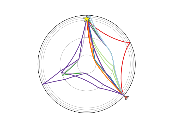
If ray paths have been calculated, they can be plotted using the
Arrivals.plot_rays() method:
>>> arrivals = model.get_ray_paths(
...     source_depth_in_km=500, distance_in_degree=130, phase_list=["ttbasic"])
>>> ax = arrivals.plot_rays()
(Source code, png)

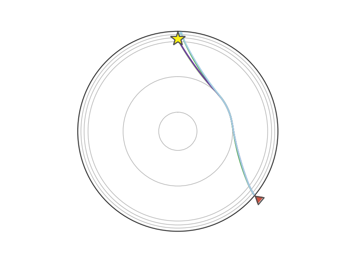
Plotting will only show the requested phases:
>>> arrivals = model.get_ray_paths(source_depth_in_km=500,
...                                distance_in_degree=130,
...                                phase_list=["Pdiff", "Sdiff",
...                                            "pPdiff", "sSdiff"])
>>> ax = arrivals.plot_rays()
(Source code, png)
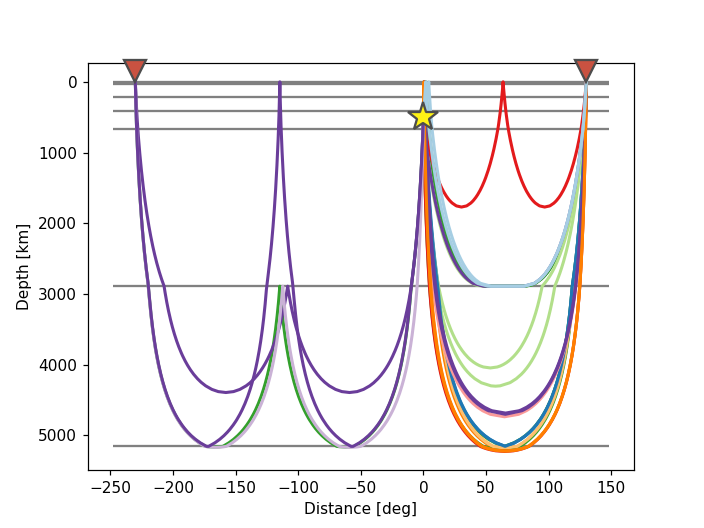
Additionally, Cartesian coordinates may be used instead of a polar grid:
>>> arrivals = model.get_ray_paths(source_depth_in_km=500,
...                                distance_in_degree=130,
...                                phase_list=["ttbasic"])
>>> ax = arrivals.plot_rays(plot_type="cartesian")
(Source code, png)

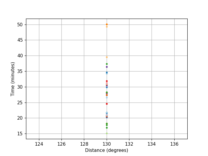
Travel times for these ray paths can be plotted using the
Arrivals.plot_times() method:
>>> arrivals = model.get_ray_paths(source_depth_in_km=500,
...                                distance_in_degree=130)
>>> ax = arrivals.plot_times()
(Source code, png)

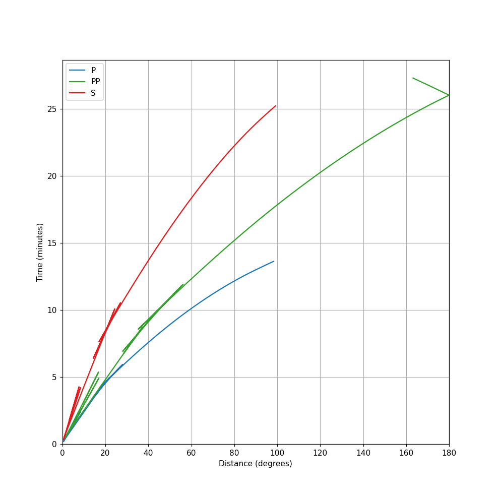
Alternatively, convenience wrapper functions plot the arrival times and the ray paths for a range of epicentral distances.
The travel times wrapper function is plot_travel_times(),
creating the figure and axes first is optional to have control over e.g. figure
size or subplot setup:
>>> from obspy.taup import plot_travel_times
>>> import matplotlib.pyplot as plt
>>> fig, ax = plt.subplots(figsize=(9, 9))
>>> ax = plot_travel_times(source_depth=10, phase_list=["P", "S", "PP"],
...                        ax=ax, fig=fig)
(Source code, png)
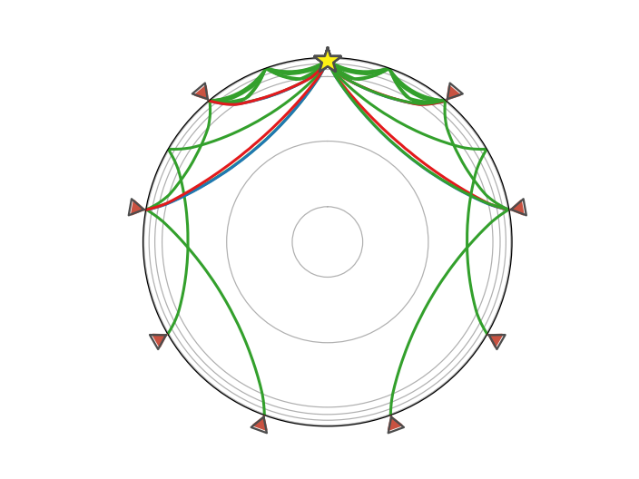
The ray path plot wrapper function is plot_ray_paths().
Again, creating the figure and axes first is optional to have control over e.g.
figure size or subplot setup (note that a polar axes has to be set up when
aiming to do a plot with plot_type='spherical' and a normal matplotlib axes
when aiming to do a plot with plot_type='cartesian'. An error will be
raised when mixing the two options):
>>> from obspy.taup import plot_ray_paths
>>> import matplotlib.pyplot as plt
>>> fig, ax = plt.subplots(subplot_kw=dict(projection='polar'))
>>> ax = plot_ray_paths(source_depth=100, ax=ax, fig=fig, verbose=True)
There were rays for all but the following epicentral distances:
 [0.0, 360.0]
(Source code, png)

More examples of plotting may be found in the ObsPy tutorial.
Phase naming in obspy.taup
Note
This section is a modified copy from the Java TauP Toolkit documentation so all credit goes to the authors of that.
A major feature of obspy.taup is the implementation of a phase name parser
that allows the user to define essentially arbitrary phases through a planet.
Thus, obspy.taup is extremely flexible in this respect since it is not
limited to a pre-defined set of phases. Phase names are not hard-coded into the
software, rather the names are interpreted and the appropriate propagation path
and resulting times are constructed at run time. Designing a phase-naming
convention that is general enough to support arbitrary phases and easy to
understand is an essential and somewhat challenging step. The rules that we
have developed are described here. Most of the phases resulting from these
conventions should be familiar to seismologists, e.g. pP, PP, PcS,
PKiKP, etc. However, the uniqueness required for parsing results in some
new names for other familiar phases.
In traditional “whole-Earth” seismology, there are 3 major interfaces: the free
surface, the core-mantle boundary, and the inner-outer core boundary. Phases
interacting with the core-mantle boundary and the inner core boundary are easy
to describe because the symbol for the wave type changes at the boundary (i.e.,
the symbol P changes to K within the outer core even though the wave
type is the same). Phase multiples for these interfaces and the free surface
are also easy to describe because the symbols describe a unique path. The
challenge begins with the description of interactions with interfaces within
the crust and upper mantle. We have introduced two new symbols to existing
nomenclature to provide unique descriptions of potential paths. Phase names are
constructed from a sequence of symbols and numbers (with no spaces) that either
describe the wave type, the interaction a wave makes with an interface, or the
depth to an interface involved in an interaction.
- Symbols that describe wave-type are:
P- compressional wave, upgoing or downgoing; in the crust or mantle,pis a strictly upgoing P-wave in the crust or mantleS- shear wave, upgoing or downgoing, in the crust or mantles- strictly upgoing S-wave in the crust or mantleK- compressional wave in the outer coreI- compressional wave in the inner coreJ- shear wave in the inner core
- Symbols that describe interactions with interfaces are:
m- interaction with the Mohogappended toPorS- ray turning in the crustnappended toPorS- head wave along the Mohoc- topside reflection off the core mantle boundaryi- topside reflection off the inner core outer core boundaryˆ- underside reflection, used primarily for crustal and mantle interfacesv- topside reflection, used primarily for crustal and mantle interfacesdiffappended toPorS- diffracted wave along the core mantle boundary; appended toK- diffracted wave along the inner-core outer-core boundarykmpsappended to a velocity - horizontal phase velocity (see 10 below)edappended toPorS- an exclusively downgoing path, for a receiver below the source (see 3 below)
The characters
pandsalways represent up-going legs. An example is the source to surface leg of the phasepPfrom a source at depth.PandScan be turning waves, but always indicate downgoing waves leaving the source when they are the first symbol in a phase name. Thus, to get near-source, direct P-wave arrival times, you need to specify two phasespandPor use the “ttimes compatibility phases” described below. However,Pmay represent a upgoing leg in certain cases. For instance,PcPis allowed since the direction of the phase is unambiguously determined by the symbolc, but would be namedPcpby a purist using our nomenclature.With the ability to have sources at depth, there is a need to specify the difference between a wave that is exclusively downgoing to the receiver from one that turns and is upgoing at the receiver. The suffix
edcan be appended to indicate exclusively downgoing. So for a source at 10 km depth and a receiver at 20 km depth at 0 degree distancePdoes not have an arrival butPeddoes.Numbers, except velocities for
kmpsphases (see 10 below), represent depths at which interactions take place. For example,P410srepresents a P-to-S conversion at a discontinuity at 410km depth. Since the S-leg is given by a lower-case symbol and no reflection indicator is included, this represents a P-wave converting to an S-wave when it hits the interface from below. The numbers given need not be the actual depth; the closest depth corresponding to a discontinuity in the model will be used. For example, if the time forP410sis requested in a model where the discontinuity was really located at 406.7 kilometers depth, the time returned would actually be forP406.7s. The code would note that this had been done. Obviously, care should be taken to ensure that there are no other discontinuities closer than the one of interest, but this approach allows generic interface names like “410” and “660” to be used without knowing the exact depth in a given model.If a number appears between two phase legs, e.g.
S410P, it represents a transmitted phase conversion, not a reflection. Thus,S410Pwould be a transmitted conversion from S to P at 410km depth. Whether the conversion occurs on the down-going side or up-going side is determined by the upper or lower case of the following leg. For instance, the phaseS410Ppropagates down as anS, converts at the 410 to aP, continues down, turns as a P-wave, and propagates back across the 410 and to the surface.S410pon the other hand, propagates down as aSthrough the 410, turns as an S-wave, hits the 410 from the bottom, converts to apand then goes up to the surface. In these cases, the case of the phase symbol (Pvs.p) is critical because the direction of propagation (upgoing or downgoing) is not unambiguously defined elsewhere in the phase name. The importance is clear when you consider a source depth below 410 compared to above 410. For a source depth greater than 410 km,S410Ptechnically cannot exist whileS410pmaintains the same path (a receiver side conversion) as it does for a source depth above the 410. The first letter can be lower case to indicate a conversion from an up-going ray, e.g.,p410Sis a depth phase from a source at greater than 410 kilometers depth that phase converts at the 410 discontinuity. It is strictly upgoing over its entire path, and hence could also be labeledp410s.p410Sis often used to mean a reflection in the literature, but there are too many possible interactions for the phase parser to allow this. If the underside reflection is desired, use thepˆ410Snotation from rule 7.Due to the two previous rules,
P410PandS410Sare over specified, but still legal. They are almost equivalent toPandS, respectively, but restrict the path to phases transmitted through (turning below) the 410. This notation is useful to limit arrivals to just those that turn deeper than a discontinuity (thus avoiding travel time curve triplications), even though they have no real interaction with it.The characters
ˆandvare new symbols introduced here to represent bottom-side and top-side reflections, respectively. They are followed by a number to represent the approximate depth of the reflection or a letter for standard discontinuities,m,cori. Reflections from discontinuities besides the core-mantle boundary,c, or inner-core outer-core boundary,i, must use theˆandvnotation. For instance, in the TauP convention,pˆ410Sis used to describe a near-source underside reflection. Underside reflections, except at the surface (PP,sS, etc.), core-mantle boundary (PKKP,SKKKS, etc.), or outer-core-inner-core boundary (PKIIKP,SKJJKS,SKIIKS, etc.), must be specified with theˆnotation. For example,Pˆ410PandPˆmPwould both be underside reflections from the 410km discontinuity and the Moho, respectively. The phasePmP, the traditional name for a top-side reflection from the Moho discontinuity, must change names under our new convention. The new name isPvmPorPvmpwhilePmPjust describes a P-wave that turns beneath the Moho. The reason why the Moho must be handled differently from the core-mantle boundary is that traditional nomenclature did not introduce a phase symbol change at the Moho. Thus, whilePcPmakes sense since a P-wave in the core would be labeledK,PmPcould have several meanings. Themsymbol just allows the user to describe phases interaction with the Moho without knowing its exact depth. In all other respects, theˆ-vnomenclature is maintained.Currently,
ˆandvfor non-standard discontinuities are allowed only in the crust and mantle. Thus there are no reflections off non-standard discontinuities within the core, (reflections such asPKKP,PKiKPandPKIIKPare still fine). There is no reason in principle to restrict reflections off discontinuities in the core, but until there is interest expressed, these phases will not be added. Also, a naming convention would have to be created since “pis toP” is not the same as “iis toI”.Currently there is no support for
PKPab,PKPbc, orPKPdfphase names. They lead to increased algorithmic complexity that at this point seems unwarranted. Currently, in regions where triplications develop, the triplicated phase will have multiple arrivals at a given distance. So,PKPabandPKPbcare both labeled justPKPwhilePKPdfis calledPKIKP.The symbol
kmpsis used to get the travel time for a specific horizontal phase velocity. For example,2kmpsrepresents a horizontal phase velocity of 2 kilometers per second. While the calculations for these are trivial, it is convenient to have them available to estimate surface wave travel times or to define windows of interest for given paths.As a convenience, a
ttimesphase name compatibility mode is available. Sottpgives you the phase list corresponding toPinttimes. Similarly there aretts,ttp+,tts+,ttbasicandttall.
Building custom models
Custom models can be built from .tvel and .nd files using the
build_taup_model() function.
Classes & Functions
Representation of a seismic model and methods for ray paths through it. |
|
The VelocityLayer dtype stores a single layer. |
|
The SlownessLayer dtype stores a single layer. |
|
Holds the ray parameter, time and distance increments, and optionally a depth, for a ray passing through some layer. |
|
Holds the ray parameter, time and distance increments, and optionally a depth, latitude and longitude for a ray passing through some layer. |
|
Tracks critical points (discontinuities or reversals in slowness gradient) within slowness and velocity models. |
Modules
C wrappers for some crucial inner loops of TauPy written in C. |
|
Holds various helper classes to keep the file number manageable. |
|
Calculations for 3D ray paths. |
|
Objects and functions dealing with seismic phases. |
|
Functions acting on slowness layers. |
|
Slowness model class. |
|
Object dealing with branches in the model. |
|
Internal TauModel class. |
|
Class to create new models. |
|
Functions to handle geographical points |
|
Ray path calculations. |
|
Pierce point calculations. |
|
Travel time calculations. |
|
High-level interface to travel-time calculation routines. |
|
Misc functionality. |
|
Functionality for dealing with a single velocity layer. |
|
Velocity model class. |