Cartopy Plots
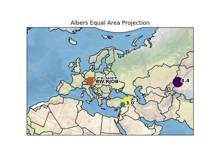
Cartopy Plot with Custom Projection Setup
Simple Cartopy plots of e.g. Inventory
or Catalog objects can be performed with
builtin methods, see e.g.
Inventory.plot() or
Catalog.plot().
For full control over the projection and map extent, a custom map can be
set up (e.g. following the examples in the
cartopy documentation),
and then be reused for plots of
e.g. Inventory or
Catalog objects:
import cartopy.crs as ccrs
import cartopy.feature as cfeature
import matplotlib.pyplot as plt

from obspy import read_inventory, read_events

# Set up a custom projection
projection = ccrs.AlbersEqualArea(
    central_longitude=35,
    central_latitude=50,
    standard_parallels=(40, 42)
)

# Set up a figure
fig = plt.figure(dpi=150)
ax = fig.add_subplot(111, projection=projection)
ax.set_extent((-15., 75., 15., 80.))

# Draw standard features
ax.gridlines()
ax.coastlines()
ax.stock_img()
ax.add_feature(cfeature.BORDERS)

ax.set_title("Albers Equal Area Projection")

# Now, let's plot some data on the map
inv = read_inventory()
inv.plot(fig=fig, show=False)
cat = read_events()
cat.plot(fig=fig, show=False, title="", colorbar=False)

plt.show()
(Source code, png)
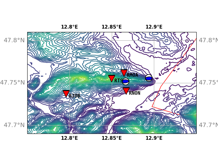
Cartopy Plot of a Local Area with Beachballs
The following example shows how to plot beachballs into a cartopy plot together with some stations. The example requires the cartopy package (pypi) to be installed. The SRTM file used can be downloaded here. The first lines of our SRTM data file (from CGIAR) look like this:
ncols         400
nrows         200
xllcorner     12°40'E
yllcorner     47°40'N
xurcorner     13°00'E
yurcorner     47°50'N
cellsize      0.00083333333333333
NODATA_value  -9999
682 681 685 690 691 689 678 670 675 680 681 679 675 671 674 680 679 679 675 671 668 664 659 660 656 655 662 666 660 659 659 658 ....
import cartopy.crs as ccrs
import cartopy.feature as cfeature
from cartopy.mpl.ticker import LongitudeFormatter, LatitudeFormatter
import gzip
import matplotlib.pyplot as plt
import matplotlib.ticker as mticker
import numpy as np

from obspy.imaging.beachball import beach


# read in topo data (on a regular lat/lon grid)
# (SRTM data from: http://srtm.csi.cgiar.org/)
with gzip.open("srtm_1240-1300E_4740-4750N.asc.gz") as fp:
    srtm = np.loadtxt(fp, skiprows=8)

# origin of data grid as stated in SRTM data file header
# create arrays with all lon/lat values from min to max and
lats = np.linspace(47.8333, 47.6666, srtm.shape[0])
lons = np.linspace(12.6666, 13.0000, srtm.shape[1])

# Prepare figure and Axis object with a proper projection and extent
projection = ccrs.PlateCarree()
fig = plt.figure(dpi=150)
ax = fig.add_subplot(111, projection=projection)
ax.set_extent((12.75, 12.95, 47.69, 47.81))

# create grids and compute map projection coordinates for lon/lat grid
grid = projection.transform_points(ccrs.Geodetic(),
                                   *np.meshgrid(lons, lats),  # unpacked x, y
                                   srtm)  # z from topo data

# Make contour plot
ax.contour(*grid.T, transform=projection, levels=30)

# Draw country borders with red
ax.add_feature(cfeature.BORDERS.with_scale('50m'), edgecolor='red')

# Draw a lon/lat grid and format the labels
gl = ax.gridlines(crs=projection, draw_labels=True)

gl.xlocator = mticker.FixedLocator([12.75, 12.8, 12.85, 12.9, 12.95])
gl.ylocator = mticker.FixedLocator([47.7, 47.75, 47.8])
gl.xformatter = LongitudeFormatter()
gl.yformatter = LatitudeFormatter()
gl.ylabel_style = {'size': 13, 'color': 'gray'}
gl.xlabel_style = {'weight': 'bold'}


# Plot station positions and names into the map
# again we have to compute the projection of our lon/lat values
lats = np.array([47.761659, 47.7405, 47.755100, 47.737167])
lons = np.array([12.864466, 12.8671, 12.849660, 12.795714])
names = [" RMOA", " RNON", " RTSH", " RJOB"]
x, y, _ = projection.transform_points(ccrs.Geodetic(), lons, lats).T
ax.scatter(x, y, 200, color="r", marker="v", edgecolor="k", zorder=3)
for i in range(len(names)):
    plt.text(x[i], y[i], names[i], va="top", family="monospace", weight="bold")

# Add beachballs for two events
lats = np.array([47.751602, 47.75577])
lons = np.array([12.866492, 12.893850])
points = projection.transform_points(ccrs.Geodetic(), lons, lats)

# Two focal mechanisms for beachball routine, specified as [strike, dip, rake]
focmecs = [[80, 50, 80], [85, 30, 90]]
for i in range(len(focmecs)):
    b = beach(focmecs[i], xy=(points[i][0], points[i][1]),
              width=0.008, linewidth=1, zorder=10)
    ax.add_collection(b)

plt.show()
(Source code, png)
Some notes:
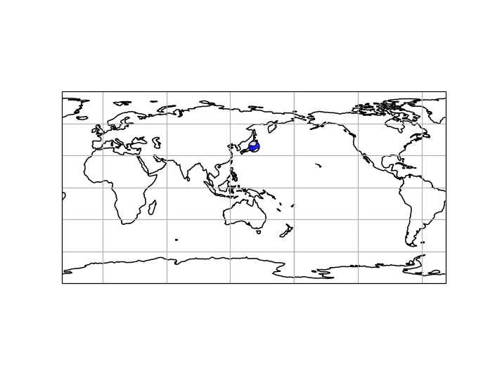
Cartopy Plot of the Globe with Beachballs
import matplotlib.pyplot as plt
import cartopy.crs as ccrs

from obspy.imaging.beachball import beach


projection = ccrs.PlateCarree(central_longitude=142.0)

fig = plt.figure(dpi=150)
ax = fig.add_subplot(111, projection=projection)
ax.set_extent((-180, 180, -90, 90))
ax.coastlines()
ax.gridlines()

x, y = projection.transform_point(x=142.36929, y=38.3215,
                                  src_crs=ccrs.Geodetic())
focmecs = [0.136, -0.591, 0.455, -0.396, 0.046, -0.615]

ax = plt.gca()
b = beach(focmecs, xy=(x, y), width=10, linewidth=1, alpha=0.85)
b.set_zorder(10)
ax.add_collection(b)

plt.show()
(Source code, png)
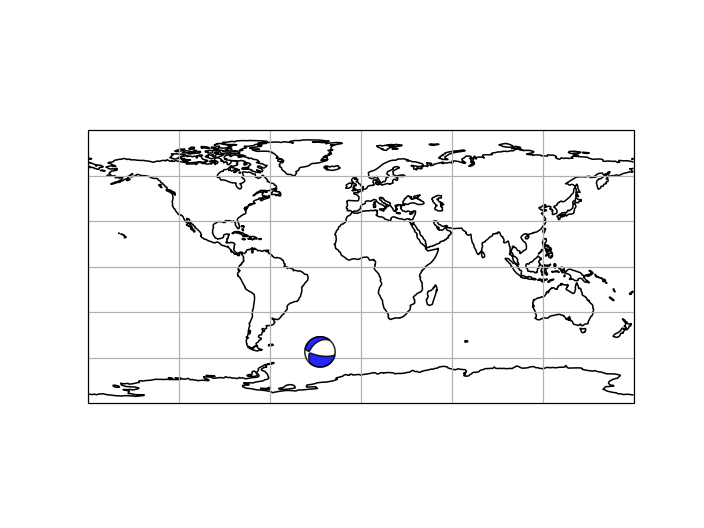
Cartopy Plot of the Globe with Beachball using read_events
import matplotlib.pyplot as plt
import cartopy.crs as ccrs

from obspy import read_events
from obspy.imaging.beachball import beach


event = read_events(
    'https://earthquake.usgs.gov/product/moment-tensor/'
    'us_20005ysu_mww/us/1470868224040/quakeml.xml', format='QUAKEML')[0]
origin = event.preferred_origin() or event.origins[0]
focmec = event.preferred_focal_mechanism() or event.focal_mechanisms[0]
tensor = focmec.moment_tensor.tensor
moment_list = [tensor.m_rr, tensor.m_tt, tensor.m_pp,
               tensor.m_rt, tensor.m_rp, tensor.m_tp]

projection = ccrs.PlateCarree(central_longitude=0.0)
x, y = projection.transform_point(x=origin.longitude, y=origin.latitude,
                                  src_crs=ccrs.Geodetic())

fig = plt.figure(dpi=150)
ax = fig.add_subplot(111, projection=projection)
ax.set_extent((-180, 180, -90, 90))
ax.coastlines()
ax.gridlines()

b = beach(moment_list, xy=(x, y), width=20, linewidth=1, alpha=0.85, zorder=10)
b.set_zorder(10)
ax.add_collection(b)

fig.show()
(Source code, png)