Trigger/Picker Tutorial
This is a small tutorial that started as a practical for the UNESCO short course on triggering. Test data used in this tutorial can be downloaded here: trigger_data.zip.
The triggers are implemented as described in [Withers1998]. Information on finding the right trigger parameters for STA/LTA type triggers can be found in [Trnkoczy2012]. The list includes (but not limited to):
Generally, STA duration must be longer than a few periods (zero-crossings of the main frequency) of a typically expected seismic signal. On the other hand, STA duration must be shorter than the shortest events (trigger on/off, the envelope duration) we expect to capture.
STA duration must be longer than the inverse frequency of noisy spikes. Otherwise, false alarms will be captured.
The LTA window should be longer than a few ‘periods’ of typically irregular (slow) seismic noise fluctuations. Typically, it’s an order of magnitude larger than the STA duration.
A nice explanation of STA and LTA parameters is given in [Han2009]:
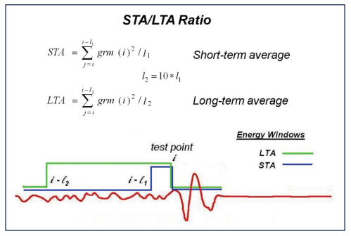
FIG. 1: Definition of the STA/LTA method. The length of the LTA energy collection window is five to ten times the length of the STA energy collection window, which needs to be on the order or two to three times the dominant period of the seismic arrival.
See also
Please note the convenience method of ObsPy’s
Stream.trigger and
Trace.trigger
objects for triggering.
Reading Waveform Data
The data files are read into an ObsPy Trace object
using the read() function.
>>> from obspy.core import read
>>> st = read("https://examples.obspy.org/ev0_6.a01.gse2")
>>> st = st.select(component="Z")
>>> tr = st[0]
The data format is automatically detected. Important in this tutorial are the
Trace attributes:
tr.datacontains the data as
numpy.ndarraytr.statscontains a dict-like class of header entries
tr.stats.sampling_ratethe sampling rate
tr.stats.nptssample count of data
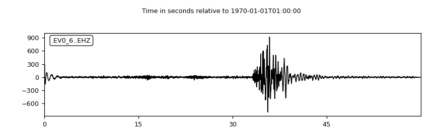
As an example, the header of the data file is printed and the data are plotted like this:
>>> print(tr.stats)
         network:
         station: EV0_6
        location:
         channel: EHZ
       starttime: 1970-01-01T01:00:00.000000Z
         endtime: 1970-01-01T01:00:59.995000Z
   sampling_rate: 200.0
           delta: 0.005
            npts: 12000
           calib: 1.0
         _format: GSE2
            gse2: AttribDict({'instype': '      ', 'datatype': 'CM6', 'hang': 0.0, 'auxid': '    ', 'vang': -1.0, 'calper': 1.0})
Using the plot() method of the
Trace objects will show the plot.
>>> tr.plot(type="relative")
(Source code, png)

Available Methods
After loading the data, we are able to pass the waveform data to the following
trigger routines defined in obspy.signal.trigger:
|
Recursive STA/LTA. |
|
Computes the carlSTAtrig characteristic function. |
|
Computes the standard STA/LTA from a given input array a. |
|
Delayed STA/LTA. |
|
Z-detector. |
|
Wrapper for P-picker routine by M. |
|
Pick P and S arrivals with an AR-AIC + STA/LTA algorithm. |
|
Energy ratio detector. |
|
Modified energy ratio detector. |
Help for each function is available HTML formatted or in the usual Python manner:
>>> from obspy.signal.trigger import classic_sta_lta
>>> help(classic_sta_lta)
Help on function classic_sta_lta in module obspy.signal.trigger...
The triggering itself mainly consists of the following two steps:
Calculating the characteristic function
Setting picks based on values of the characteristic function
Trigger Examples
For all the examples, the commands to read in the data and to load the modules are the following:
>>> import matplotlib.pyplot as plt
>>> from obspy.core import read
>>> from obspy.signal.trigger import plot_trigger, plot_trace
>>> trace = read("https://examples.obspy.org/ev0_6.a01.gse2")[0]
>>> df = trace.stats.sampling_rate
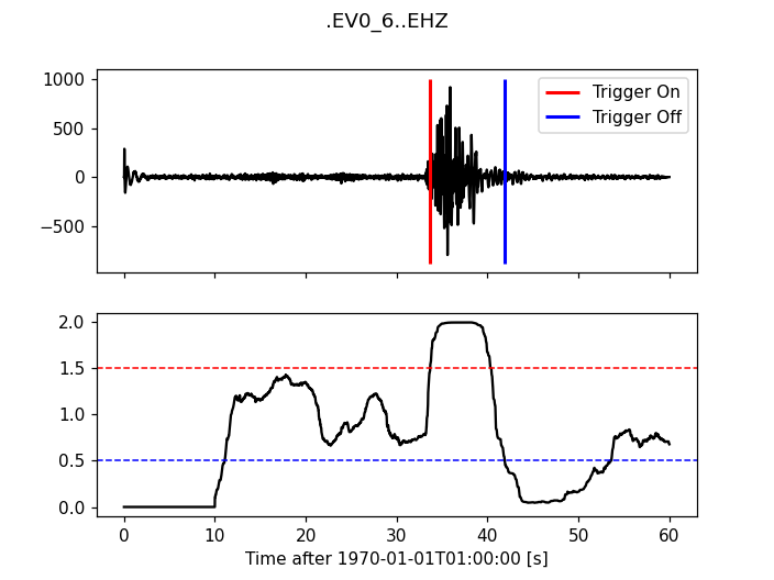
Classic Sta Lta
>>> from obspy.signal.trigger import classic_sta_lta
>>> cft = classic_sta_lta(trace.data, int(5 * df), int(10 * df))
>>> plot_trigger(trace, cft, 1.5, 0.5)
(Source code, png)
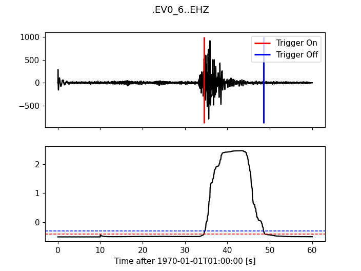
Z-Detect
>>> from obspy.signal.trigger import z_detect
>>> cft = z_detect(trace.data, int(10 * df))
>>> plot_trigger(trace, cft, -0.4, -0.3)
(Source code, png)
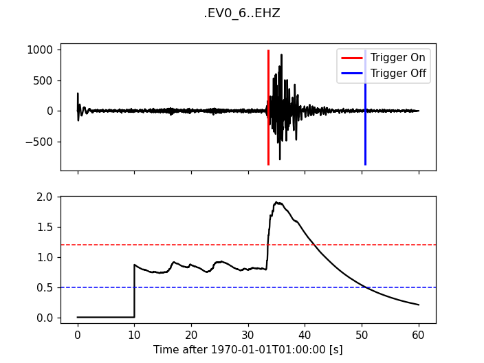
Recursive Sta Lta
>>> from obspy.signal.trigger import recursive_sta_lta
>>> cft = recursive_sta_lta(trace.data, int(5 * df), int(10 * df))
>>> plot_trigger(trace, cft, 1.2, 0.5)
(Source code, png)

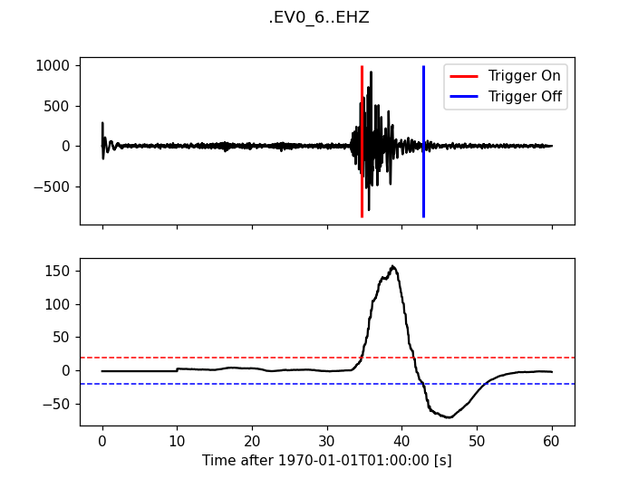
Carl-Sta-Trig
>>> from obspy.signal.trigger import carl_sta_trig
>>> cft = carl_sta_trig(trace.data, int(5 * df), int(10 * df), 0.8, 0.8)
>>> plot_trigger(trace, cft, 20.0, -20.0)
(Source code, png)
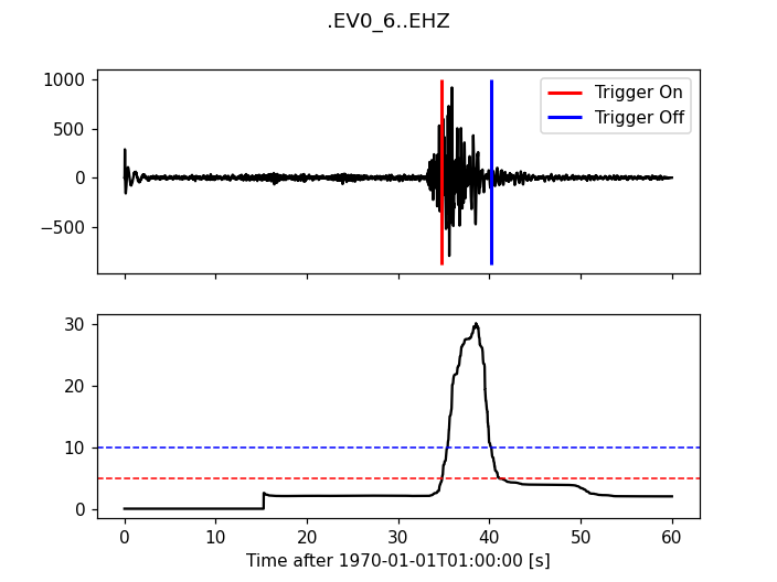
Delayed Sta Lta
>>> from obspy.signal.trigger import delayed_sta_lta
>>> cft = delayed_sta_lta(trace.data, int(5 * df), int(10 * df))
>>> plot_trigger(trace, cft, 5, 10)
(Source code, png)
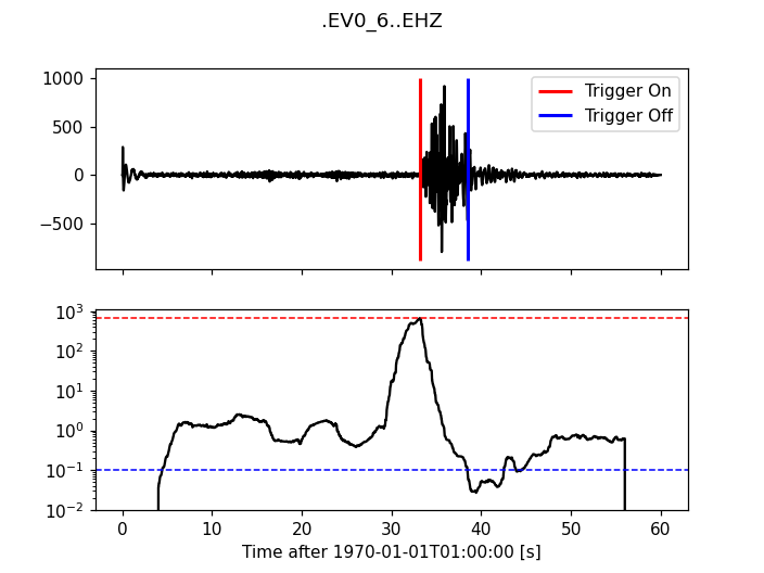
Energy Ratio
import matplotlib.pyplot as plt

import obspy
from obspy.signal.trigger import plot_trigger, energy_ratio


trace = obspy.read("https://examples.obspy.org/ev0_6.a01.gse2")[0]
df = trace.stats.sampling_rate

cft = energy_ratio(trace.data, int(4 * df))
fig, axes = plot_trigger(trace, cft, cft.max(), 0.1, show=False)
axes[1].set_yscale('log')
axes[1].set_ylim(ymin=0.01)
plt.show()
(Source code, png)
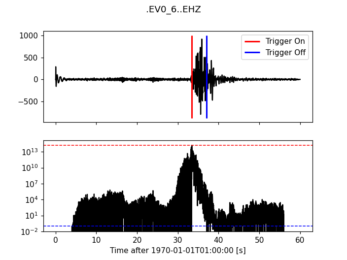
Modified Energy Ratio
An improvement of the energy ratio that accounts for the signal itself.
The picture below is taken from [Han2009].
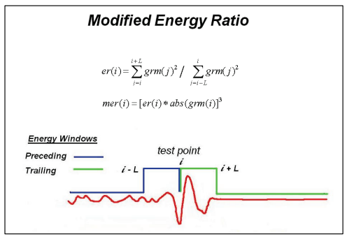
FIG. 2: Definition of the MER method. Preceding and following energy collection windows with equal lengths are located at a test point. The window lengths are two to three times the dominant periods of the seismic arrival.
import matplotlib.pyplot as plt

import obspy
from obspy.signal.trigger import plot_trigger, modified_energy_ratio


trace = obspy.read("https://examples.obspy.org/ev0_6.a01.gse2")[0]
df = trace.stats.sampling_rate

cft = modified_energy_ratio(trace.data, int(4 * df))
fig, axes = plot_trigger(trace, cft, cft.max(), 0.1, show=False)
axes[1].set_yscale('log')
axes[1].set_ylim(ymin=0.01)
plt.show()
(Source code, png)

Network Coincidence Trigger Example
In this example we perform a coincidence trigger on a local scale network of 4 stations. For the single station triggers a recursive STA/LTA is used. The waveform data span about four minutes and include four local events. Two are easily recognizable (Ml 1-2), the other two can only be detected with well adjusted trigger settings (Ml <= 0).
First we assemble a Stream object with all waveform data, the data used in the example is available from our web server:
>>> from obspy.core import Stream, read
>>> st = Stream()
>>> files = ["BW.UH1..SHZ.D.2010.147.cut.slist.gz",
...          "BW.UH2..SHZ.D.2010.147.cut.slist.gz",
...          "BW.UH3..SHZ.D.2010.147.cut.slist.gz",
...          "BW.UH4..SHZ.D.2010.147.cut.slist.gz"]
>>> for filename in files:
...     st += read("https://examples.obspy.org/" + filename)
After applying a bandpass filter we run the coincidence triggering on all data. In the example a recursive STA/LTA is used. The trigger parameters are set to 0.5 and 10 second time windows, respectively. The on-threshold is set to 3.5, the off-threshold to 1. In this example every station gets a weight of 1 and the coincidence sum threshold is set to 3. For more complex network setups the weighting for every station/channel can be customized. We want to keep our original data so we work with a copy of the original stream:
>>> st.filter('bandpass', freqmin=10, freqmax=20)  # optional prefiltering
>>> from obspy.signal.trigger import coincidence_trigger
>>> st2 = st.copy()
>>> trig = coincidence_trigger("recstalta", 3.5, 1, st2, 3, sta=0.5, lta=10)
Using pretty print the results display like this:
>>> from pprint import pprint
>>> pprint(trig)
[{'coincidence_sum': 4.0,
  'duration': 4.5299999713897705,
  'stations': ['UH3', 'UH2', 'UH1', 'UH4'],
  'time': UTCDateTime(2010, 5, 27, 16, 24, 33, 190000),
  'trace_ids': ['BW.UH3..SHZ', 'BW.UH2..SHZ', 'BW.UH1..SHZ',
                'BW.UH4..SHZ']},
 {'coincidence_sum': 3.0,
  'duration': 3.440000057220459,
  'stations': ['UH2', 'UH3', 'UH1'],
  'time': UTCDateTime(2010, 5, 27, 16, 27, 1, 260000),
  'trace_ids': ['BW.UH2..SHZ', 'BW.UH3..SHZ', 'BW.UH1..SHZ']},
 {'coincidence_sum': 4.0,
  'duration': 4.7899999618530273,
  'stations': ['UH3', 'UH2', 'UH1', 'UH4'],
  'time': UTCDateTime(2010, 5, 27, 16, 27, 30, 490000),
  'trace_ids': ['BW.UH3..SHZ', 'BW.UH2..SHZ', 'BW.UH1..SHZ',
                'BW.UH4..SHZ']}]
With these settings the coincidence trigger reports three events. For each
(possible) event the start time and duration is provided. Furthermore, a list
of station names and trace IDs is provided, ordered by the time the stations
have triggered, which can give a first rough idea of the possible event
location. We can request additional information by specifying details=True:
>>> st2 = st.copy()
>>> trig = coincidence_trigger("recstalta", 3.5, 1, st2, 3, sta=0.5, lta=10,
...                           details=True)
For clarity, we only display information on the first item in the results here:
>>> pprint(trig[0])
{'cft_peak_wmean': 19.561900329259956,
 'cft_peaks': [19.535644192544272,
               19.872432918501264,
               19.622171410201297,
               19.217352795792998],
 'cft_std_wmean': 5.4565629691954713,
 'cft_stds': [5.292458320417178,
              5.6565387957966404,
              5.7582248973698507,
              5.1190298631982163],
 'coincidence_sum': 4.0,
 'duration': 4.5299999713897705,
 'stations': ['UH3', 'UH2', 'UH1', 'UH4'],
 'time': UTCDateTime(2010, 5, 27, 16, 24, 33, 190000),
 'trace_ids': ['BW.UH3..SHZ', 'BW.UH2..SHZ', 'BW.UH1..SHZ', 'BW.UH4..SHZ']}
Here, some additional information on the peak values and standard deviations of the characteristic functions of the single station triggers is provided. Also, for both a weighted mean is calculated. These values can help to distinguish certain from questionable network triggers.
For more information on all possible options see the documentation page for
coincidence_trigger().
Advanced Network Coincidence Trigger Example with Similarity Detection
This example is an extension of the common network coincidence trigger. Waveforms with already known event(s) can be provided to check waveform similarity of single-station triggers. If the corresponding similarity threshold is exceeded the event trigger is included in the result list even if the coincidence sum does not exceed the specified minimum coincidence sum. Using this approach, events can be detected that have good recordings on one station with very similar waveforms but for some reason are not detected on enough other stations (e.g. temporary station outages or local high noise levels etc.). An arbitrary number of template waveforms can be provided for any station. Computation time might get significantly higher due to the necessary cross correlations. In the example we use two three-component event templates on top of a common network trigger on vertical components only.
>>> from obspy.core import Stream, read, UTCDateTime
>>> st = Stream()
>>> files = ["BW.UH1..SHZ.D.2010.147.cut.slist.gz",
...          "BW.UH2..SHZ.D.2010.147.cut.slist.gz",
...          "BW.UH3..SHZ.D.2010.147.cut.slist.gz",
...          "BW.UH3..SHN.D.2010.147.cut.slist.gz",
...          "BW.UH3..SHE.D.2010.147.cut.slist.gz",
...          "BW.UH4..SHZ.D.2010.147.cut.slist.gz"]
>>> for filename in files:
...     st += read("https://examples.obspy.org/" + filename)
>>> st.filter('bandpass', freqmin=10, freqmax=20)  # optional prefiltering
Here we set up a dictionary with template events for one single station. The specified times are exact P wave onsets, the event duration (including S wave) is about 2.5 seconds. On station UH3 we use two template events with three-component data, on station UH1 we use one template event with only vertical component data.
>>> times = ["2010-05-27T16:24:33.095000", "2010-05-27T16:27:30.370000"]
>>> event_templates = {"UH3": []}
>>> for t in times:
...     t = UTCDateTime(t)
...     st_ = st.select(station="UH3").slice(t, t + 2.5)
...     event_templates["UH3"].append(st_)
>>> t = UTCDateTime("2010-05-27T16:27:30.574999")
>>> st_ = st.select(station="UH1").slice(t, t + 2.5)
>>> event_templates["UH1"] = [st_]
The triggering step, including providing of similarity threshold and event template waveforms. Note that the coincidence sum is set to 4 and we manually specify to only use vertical components with equal station coincidence values of 1.
>>> from obspy.signal.trigger import coincidence_trigger
>>> st2 = st.copy()
>>> trace_ids = {"BW.UH1..SHZ": 1,
...              "BW.UH2..SHZ": 1,
...              "BW.UH3..SHZ": 1,
...              "BW.UH4..SHZ": 1}
>>> similarity_thresholds = {"UH1": 0.8, "UH3": 0.7}
>>> trig = coincidence_trigger("classicstalta", 5, 1, st2, 4, sta=0.5,
...                           lta=10, trace_ids=trace_ids,
...                           event_templates=event_templates,
...                           similarity_threshold=similarity_thresholds)
The results now include two event triggers, that do not reach the specified minimum coincidence threshold but that have a similarity value that exceeds the specified similarity threshold when compared to at least one of the provided event template waveforms. Note the values of 1.0 when checking the event triggers where we extracted the event templates for this example.
>>> from pprint import pprint
>>> pprint(trig)
[{'coincidence_sum': 4.0,
  'duration': 4.1100001335144043,
  'similarity': {'UH1': 0.9414944738498271, 'UH3': 1.0},
  'stations': ['UH3', 'UH2', 'UH1', 'UH4'],
  'time': UTCDateTime(2010, 5, 27, 16, 24, 33, 210000),
  'trace_ids': ['BW.UH3..SHZ', 'BW.UH2..SHZ', 'BW.UH1..SHZ', 'BW.UH4..SHZ']},
 {'coincidence_sum': 3.0,
  'duration': 1.9900000095367432,
  'similarity': {'UH1': 0.65228204570577764, 'UH3': 0.72679293429214198},
  'stations': ['UH3', 'UH1', 'UH2'],
  'time': UTCDateTime(2010, 5, 27, 16, 25, 26, 710000),
  'trace_ids': ['BW.UH3..SHZ', 'BW.UH1..SHZ', 'BW.UH2..SHZ']},
 {'coincidence_sum': 3.0,
  'duration': 1.9200000762939453,
  'similarity': {'UH1': 0.89404458774338103, 'UH3': 0.74581409371425222},
  'stations': ['UH2', 'UH1', 'UH3'],
  'time': UTCDateTime(2010, 5, 27, 16, 27, 2, 260000),
  'trace_ids': ['BW.UH2..SHZ', 'BW.UH1..SHZ', 'BW.UH3..SHZ']},
 {'coincidence_sum': 4.0,
  'duration': 4.0299999713897705,
  'similarity': {'UH1': 1.0, 'UH3': 1.0},
  'stations': ['UH3', 'UH2', 'UH1', 'UH4'],
  'time': UTCDateTime(2010, 5, 27, 16, 27, 30, 510000),
  'trace_ids': ['BW.UH3..SHZ', 'BW.UH2..SHZ', 'BW.UH1..SHZ', 'BW.UH4..SHZ']}]
For more information on all possible options see the documentation page for
coincidence_trigger().
Picker Examples
Baer Picker
For pk_baer(), input is in seconds, output is in
samples.
>>> from obspy.core import read
>>> from obspy.signal.trigger import pk_baer
>>> trace = read("https://examples.obspy.org/ev0_6.a01.gse2")[0]
>>> df = trace.stats.sampling_rate
>>> p_pick, phase_info = pk_baer(trace.data, df,
...                             20, 60, 7.0, 12.0, 100, 100)
>>> print(p_pick)
6894
>>> print(phase_info)
EPU3
>>> print(p_pick / df)
34.47
This yields the output 34.47 EPU3, which means that a P pick was set at 34.47s with Phase information EPU3.
AR Picker
For ar_pick(), input and output are in seconds.
>>> from obspy.core import read
>>> from obspy.signal.trigger import ar_pick
>>> tr1 = read('https://examples.obspy.org/loc_RJOB20050801145719850.z.gse2')[0]
>>> tr2 = read('https://examples.obspy.org/loc_RJOB20050801145719850.n.gse2')[0]
>>> tr3 = read('https://examples.obspy.org/loc_RJOB20050801145719850.e.gse2')[0]
>>> df = tr1.stats.sampling_rate
>>> p_pick, s_pick = ar_pick(tr1.data, tr2.data, tr3.data, df,
...                          1.0, 20.0, 1.0, 0.1, 4.0, 1.0, 2, 8, 0.1, 0.2)
>>> print(p_pick)
30.6350002289
>>> print(s_pick)
31.2800006866
This gives the output 30.6350002289 and 31.2800006866, meaning that a P pick at 30.64s and an S pick at 31.28s were identified.
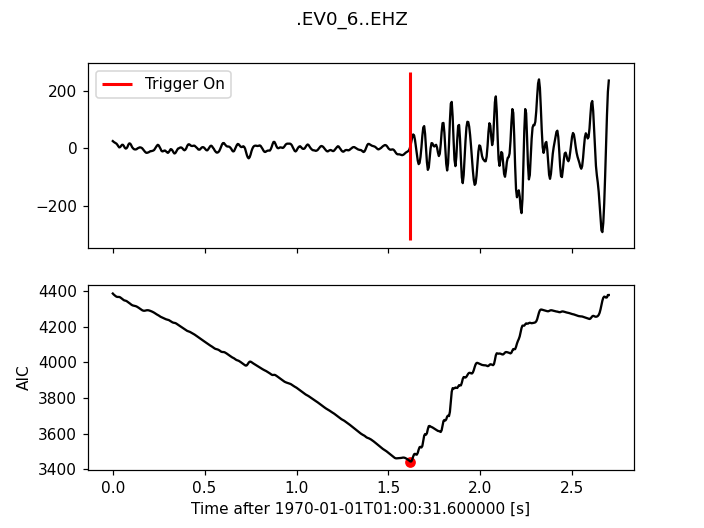
AIC - Akaike Information Criterion by Maeda (1985)
Credits: mbagagli
The aic_simple() function estimates the Akaike
Information directly from data (see [Maeda1985]). The algorithm provides a
simple way to localize points of interest, i.e. trigger onset.
(Source code, png)

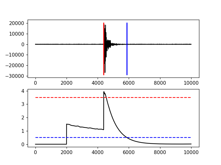
Advanced Example
A more complicated example, where the data are retrieved via FDSNWS and results are plotted step by step, is shown here:
import matplotlib.pyplot as plt

import obspy
from obspy.clients.fdsn import Client
from obspy.signal.trigger import recursive_sta_lta, trigger_onset


# Retrieve waveforms via FDSNWS
client = Client("LMU")
t = obspy.UTCDateTime("2009-08-24 00:19:45")
st = client.get_waveforms('BW', 'RTSH', '', 'EHZ', t, t + 50)

# For convenience
tr = st[0]  # only one trace in mseed volume
df = tr.stats.sampling_rate

# Characteristic function and trigger onsets
cft = recursive_sta_lta(tr.data, int(2.5 * df), int(10. * df))
on_of = trigger_onset(cft, 3.5, 0.5)

# Plotting the results
ax = plt.subplot(211)
plt.plot(tr.data, 'k')
ymin, ymax = ax.get_ylim()
plt.vlines(on_of[:, 0], ymin, ymax, color='r', linewidth=2)
plt.vlines(on_of[:, 1], ymin, ymax, color='b', linewidth=2)
plt.subplot(212, sharex=ax)
plt.plot(cft, 'k')
plt.hlines([3.5, 0.5], 0, len(cft), color=['r', 'b'], linestyle='--')
plt.axis('tight')
plt.show()
(Source code, png)