Continuous Wavelet Transform
Using ObsPy
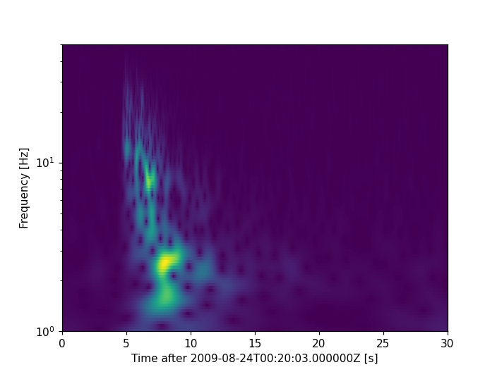
The following is a short example for a continuous wavelet transform using ObsPy’s internal routine based on [Kristekova2006].
import numpy as np
import matplotlib.pyplot as plt

import obspy
from obspy.imaging.cm import obspy_sequential
from obspy.signal.tf_misfit import cwt


st = obspy.read()
tr = st[0]
npts = tr.stats.npts
dt = tr.stats.delta
t = np.linspace(0, dt * npts, npts)
f_min = 1
f_max = 50

scalogram = cwt(tr.data, dt, 8, f_min, f_max)

fig = plt.figure()
ax = fig.add_subplot(111)

x, y = np.meshgrid(
    t,
    np.logspace(np.log10(f_min), np.log10(f_max), scalogram.shape[0]))

ax.pcolormesh(x, y, np.abs(scalogram), cmap=obspy_sequential)
ax.set_xlabel("Time after %s [s]" % tr.stats.starttime)
ax.set_ylabel("Frequency [Hz]")
ax.set_yscale('log')
ax.set_ylim(f_min, f_max)
plt.show()
(Source code, png)
Using MLPY
Small script doing the continuous wavelet transform using the mlpy package (version 3.5.0) for infrasound data recorded at Yasur in 2008. Further details on wavelets can be found at Wikipedia - in the article the omega0 factor is denoted as sigma. (really sloppy and possibly incorrect: the omega0 factor tells you how often the wavelet fits into the time window, dj defines the spacing in the scale domain)
import numpy as np
import matplotlib.pyplot as plt
try:
    import mlpy
except ModuleNotFoundError:
    import warnings
    warnings.warn("mlpy not installed, code snippet skipped")
    exit(1)

import obspy
from obspy.imaging.cm import obspy_sequential


tr = obspy.read("https://examples.obspy.org/a02i.2008.240.mseed")[0]

omega0 = 8
wavelet_fct = "morlet"
scales = mlpy.wavelet.autoscales(N=len(tr.data), dt=tr.stats.delta, dj=0.05,
                                 wf=wavelet_fct, p=omega0)
spec = mlpy.wavelet.cwt(tr.data, dt=tr.stats.delta, scales=scales,
                        wf=wavelet_fct, p=omega0)
# approximate scales through frequencies
freq = (omega0 + np.sqrt(2.0 + omega0 ** 2)) / (4 * np.pi * scales[1:])

fig = plt.figure()
ax1 = fig.add_axes([0.1, 0.75, 0.7, 0.2])
ax2 = fig.add_axes([0.1, 0.1, 0.7, 0.60], sharex=ax1)
ax3 = fig.add_axes([0.83, 0.1, 0.03, 0.6])

t = np.arange(tr.stats.npts) / tr.stats.sampling_rate
ax1.plot(t, tr.data, 'k')

img = ax2.imshow(np.abs(spec), extent=[t[0], t[-1], freq[-1], freq[0]],
                 aspect='auto', interpolation='nearest', cmap=obspy_sequential)
# Hackish way to overlay a logarithmic scale over a linearly scaled image.
twin_ax = ax2.twinx()
twin_ax.set_yscale('log')
twin_ax.set_xlim(t[0], t[-1])
twin_ax.set_ylim(freq[-1], freq[0])
ax2.tick_params(which='both', labelleft=False, left=False)
twin_ax.tick_params(which='both', labelleft=True, left=True, labelright=False)

fig.colorbar(img, cax=ax3)

plt.show()