Time Frequency Misfit
The tf_misfit module offers various Time Frequency Misfit
Functions based on [Kristekova2006] and [Kristekova2009].
Here are some examples how to use the included plotting tools:
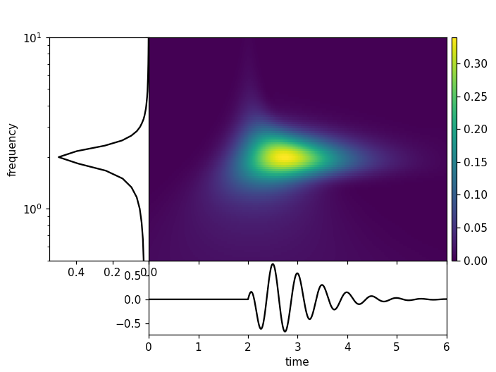
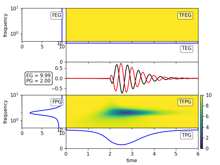
Plot the Time Frequency Representation
import numpy as np

from obspy.signal.tf_misfit import plot_tfr


# general constants
tmax = 6.
dt = 0.01
npts = int(tmax / dt + 1)
t = np.linspace(0., tmax, npts)

fmin = .5
fmax = 10

# constants for the signal
A1 = 4.
t1 = 2.
f1 = 2.
phi1 = 0.

# generate the signal
H1 = (np.sign(t - t1) + 1) / 2
st1 = A1 * (t - t1) * np.exp(-2 * (t - t1))
st1 *= np.cos(2. * np.pi * f1 * (t - t1) + phi1 * np.pi) * H1

plot_tfr(st1, dt=dt, fmin=fmin, fmax=fmax)
(Source code, png)
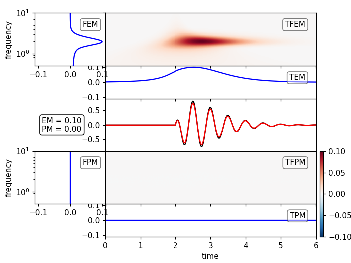
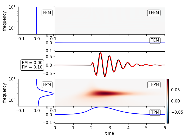
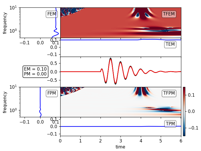
Plot the Time Frequency Misfits
Time Frequency Misfits are appropriate for smaller differences of the signals. Continuing the example from above:
from scipy.signal import hilbert
from obspy.signal.tf_misfit import plot_tf_misfits

# amplitude and phase error
phase_shift = 0.1
amp_fac = 1.1

# reference signal
st2 = st1.copy()

# generate analytical signal (hilbert transform) and add phase shift
st1p = hilbert(st1)
st1p = np.real(np.abs(st1p) * \
        np.exp((np.angle(st1p) + phase_shift * np.pi) * 1j))

# signal with amplitude error
st1a = st1 * amp_fac

plot_tf_misfits(st1a, st2, dt=dt, fmin=fmin, fmax=fmax, show=False)
plot_tf_misfits(st1p, st2, dt=dt, fmin=fmin, fmax=fmax, show=False)

plt.show()

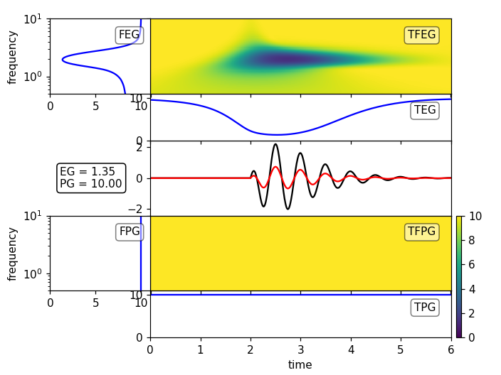
Plot the Time Frequency Goodness-Of-Fit
Time Frequency GOFs are appropriate for large differences of the signals. Continuing the example from above:
from obspy.signal.tf_misfit import plot_tf_gofs

# amplitude and phase error
phase_shift = 0.8
amp_fac = 3.

# generate analytical signal (hilbert transform) and add phase shift
st1p = hilbert(st1)
st1p = np.real(np.abs(st1p) * \
        np.exp((np.angle(st1p) + phase_shift * np.pi) * 1j))

# signal with amplitude error
st1a = st1 * amp_fac

plot_tf_gofs(st1a, st2, dt=dt, fmin=fmin, fmax=fmax, show=False)
plot_tf_gofs(st1p, st2, dt=dt, fmin=fmin, fmax=fmax, show=False)

plt.show()
Multi Component Data
For multi component data and global normalization of the misfits, the axes are scaled accordingly. Continuing the example from above:
# amplitude error
amp_fac = 1.1

# reference signals
st2_1 = st1.copy()
st2_2 = st1.copy() * 5.
st2 = np.c_[st2_1, st2_2].T

# signals with amplitude error
st1a = st2 * amp_fac

plot_tf_misfits(st1a, st2, dt=dt, fmin=fmin, fmax=fmax)
Local normalization
Local normalization allows to resolve frequency and time ranges away from the largest amplitude waves, but tend to produce artifacts in regions where there is no energy at all. In this analytical example e.g. for the high frequencies before the onset of the signal. Manual setting of the limits is thus necessary:
# amplitude and phase error
amp_fac = 1.1

ste = 0.001 * A1 * np.exp(- (10 * (t - 2. * t1)) ** 2) \

# reference signal
st2 = st1.copy()

# signal with amplitude error + small additional pulse aftert 4 seconds
st1a = st1 * amp_fac + ste

plot_tf_misfits(st1a, st2, dt=dt, fmin=fmin, fmax=fmax, show=False)
plot_tf_misfits(st1a, st2, dt=dt, fmin=fmin, fmax=fmax, norm='local',
              clim=0.15, show=False)

plt.show()

