Waveform Plotting Tutorial

Read the files as shown at the Reading Seismograms page. We will use two different ObsPy Stream objects throughout this tutorial. The first one, singlechannel, just contains one continuous Trace and the other one, threechannel, contains three channels of a seismograph.

>>> from obspy.core import read
>>> singlechannel = read('https://examples.obspy.org/COP.BHZ.DK.2009.050')
>>> print(singlechannel)
1 Trace(s) in Stream:
DK.COP..BHZ | 2009-02-19T00:00:00.025100Z - 2009-02-19T23:59:59.975100Z | 20.0 Hz, 1728000 samples

>>> threechannels = read('https://examples.obspy.org/COP.BHE.DK.2009.050')
>>> threechannels += read('https://examples.obspy.org/COP.BHN.DK.2009.050')
>>> threechannels += read('https://examples.obspy.org/COP.BHZ.DK.2009.050')
>>> print(threechannels)
3 Trace(s) in Stream:
DK.COP..BHE | 2009-02-19T00:00:00.035100Z - 2009-02-19T23:59:59.985100Z | 20.0 Hz, 1728000 samples
DK.COP..BHN | 2009-02-19T00:00:00.025100Z - 2009-02-19T23:59:59.975100Z | 20.0 Hz, 1728000 samples
DK.COP..BHZ | 2009-02-19T00:00:00.025100Z - 2009-02-19T23:59:59.975100Z | 20.0 Hz, 1728000 samples

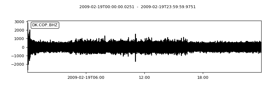
Basic Plotting

Using the plot() method of the Stream objects will show the plot. The default size of the plots is 800x250 pixel. Use the size attribute to adjust it to your needs.

>>> singlechannel.plot()

(Source code, png)

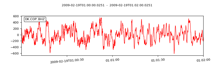
Customized Plots

This example shows the options to adjust the color of the graph, the number of ticks shown, their format and rotation and how to set the start and end time of the plot. Please see the documentation of method plot() for more details on all parameters.

>>> dt = singlechannel[0].stats.starttime
>>> singlechannel.plot(color='red', tick_rotation=5, tick_format='%I:%M %p',
...                    starttime=dt + 60*60, endtime=dt + 60*60 + 120)

(Source code, png)

Saving Plot to File

Plots may be saved into the file system by the outfile parameter. The format is determined automatically from the filename. Supported file formats depend on your matplotlib backend. Most backends support png, pdf, ps, eps and svg.

>>> singlechannel.plot(outfile='singlechannel.png')

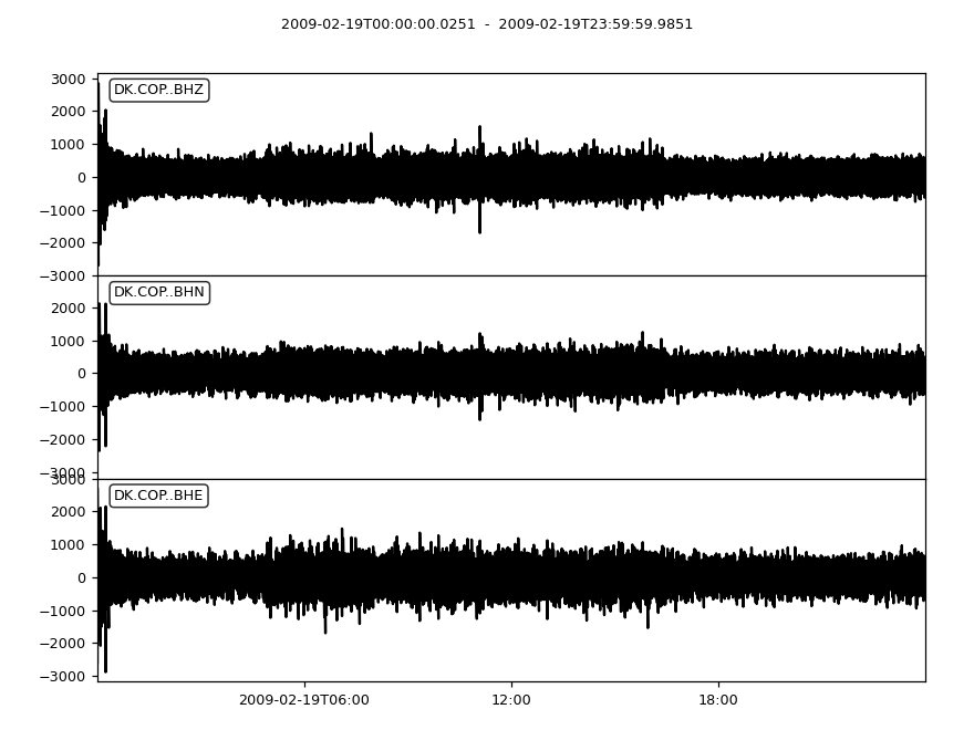
Plotting multiple Channels

If the Stream object contains more than one Trace, each Trace will be plotted in a subplot. The start- and endtime of each trace will be the same and the range on the y-axis will also be identical on each trace. Each additional subplot will add 250 pixel to the height of the resulting plot. The size attribute is used in the following example to change the overall size of the plot.

>>> threechannels.plot(size=(800, 600))

(Source code, png)

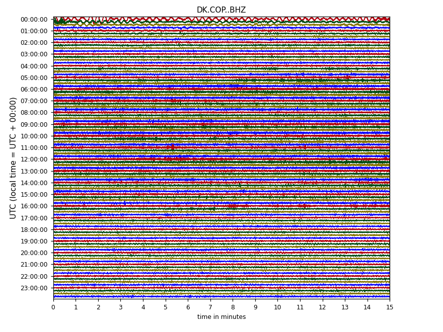
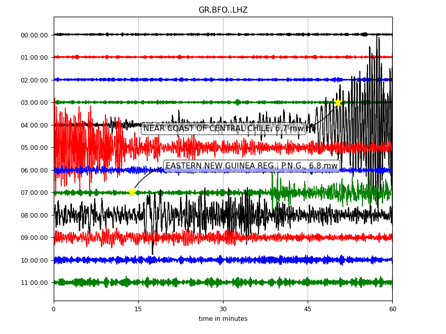
Creating a One-Day Plot

A day plot of a Trace object may be plotted by setting the type parameter to 'dayplot':

>>> singlechannel.plot(type='dayplot')

(Source code, png)

Event information can be included in the plot as well (experimental feature, syntax might change):

>>> from obspy import read
>>> st = read("https://examples.obspy.org/GR.BFO..LHZ.2012.108")
>>> st.filter("lowpass", freq=0.1, corners=2)
>>> st.plot(type="dayplot", interval=60, right_vertical_labels=False,
...         vertical_scaling_range=5e3, one_tick_per_line=True,
...         color=['k', 'r', 'b', 'g'], show_y_UTC_label=False,
...         events={'min_magnitude': 6.5})

(Source code, png)

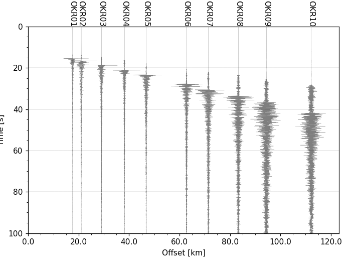
Plotting a Record Section

A record section can be plotted from a Stream object by setting parameter type to 'section':

>>> stream.plot(type='section')

To plot a record section the ObsPy header trace.stats.distance (Offset) must be defined in meters. Or a geographical location trace.stats.coordinates.latitude & trace.stats.coordinates.longitude must be defined if the section is plotted in great circle distances (dist_degree=True) along with parameter ev_coord. For further information please see plot()

(Source code, png)

Plot & Color Options

Various options are available to change the appearance of the waveform plot. Please see plot() method for all possible options.

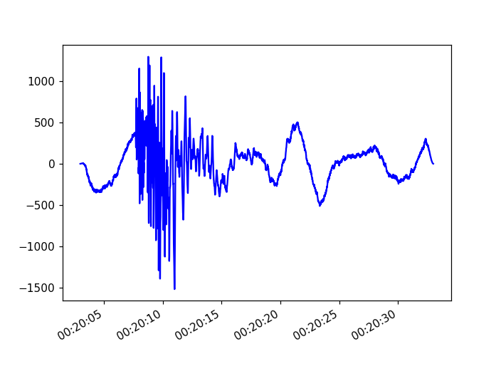
Custom Plotting using Matplotlib

Custom plots can be done using matplotlib, like shown in this minimalistic example (see http://matplotlib.org/gallery.html for more advanced plotting examples):

import matplotlib.pyplot as plt
from obspy import read

st = read()
tr = st[0]

fig = plt.figure()
ax = fig.add_subplot(1, 1, 1)
ax.plot(tr.times("matplotlib"), tr.data, "b-")
ax.xaxis_date()
fig.autofmt_xdate()
plt.show()

(Source code, png)