Visualizing Probabilistic Power Spectral Densities
The following code example shows how to use the
PPSD class defined in
obspy.signal. The routine is useful for interpretation of e.g. noise
measurements for site quality control checks. For more information on the topic
see [McNamara2004].
>>> from obspy import read
>>> from obspy.io.xseed import Parser
>>> from obspy.signal import PPSD
Read data and select a trace with the desired station/channel combination:
>>> st = read("https://examples.obspy.org/BW.KW1..EHZ.D.2011.037")
>>> tr = st.select(id="BW.KW1..EHZ")[0]
Metadata can be provided as an
Inventory (e.g. from a StationXML file
or from a request to a FDSN web service – be sure to use level=’response’),
a Parser (mostly legacy, dataless SEED files
can be read into Inventory objects using
read_inventory()), a filename of a
local RESP file (also legacy, RESP files can be parsed into Inventory
objects; or a legacy poles and zeros dictionary). Then we
initialize a new PPSD instance. The
ppsd object will then make sure that only appropriate data go into the
probabilistic psd statistics.
>>> inv = read_inventory("https://examples.obspy.org/BW_KW1.xml")
>>> ppsd = PPSD(tr.stats, metadata=inv)
Now we can add data (either trace or stream objects) to the ppsd estimate. This
step may take a while. The return value True indicates that the data was
successfully added to the ppsd estimate.
>>> ppsd.add(st)
True
We can check what time ranges are represented in the ppsd estimate.
ppsd.times_processed contains a sorted list of start times of the one hour
long slices that the psds are computed from (here only the first two are
printed). Other attributes storing information about the data fed into the
PPSD object are ppsd.times_data and ppsd.times_gaps.
>>> print(ppsd.times_processed[:2])
[UTCDateTime(2011, 2, 6, 0, 0, 0, 935000), UTCDateTime(2011, 2, 6, 0, 30, 0, 935000)]
>>> print("number of psd segments:", len(ppsd.times_processed))
number of psd segments: 47
Adding the same stream again will do nothing (return value False), the ppsd
object makes sure that no overlapping data segments go into the ppsd estimate.
>>> ppsd.add(st)
False
>>> print("number of psd segments:", len(ppsd.times_processed))
number of psd segments: 47
Additional information from other files/sources can be added step by step.
>>> st = read("https://examples.obspy.org/BW.KW1..EHZ.D.2011.038")
>>> ppsd.add(st)
True
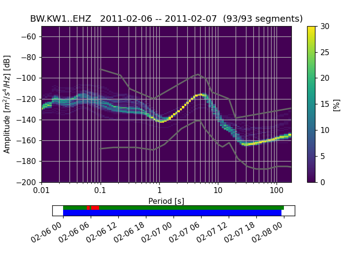
The graphical representation of the ppsd can be displayed in a matplotlib window..
>>> ppsd.plot()
..or saved to an image file:
>>> ppsd.plot("/tmp/ppsd.png")
>>> ppsd.plot("/tmp/ppsd.pdf")
(Source code, png)
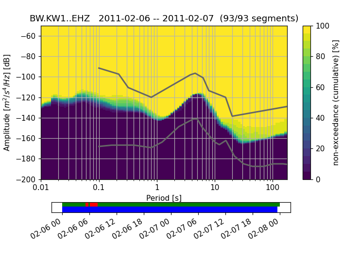
A (for each frequency bin) cumulative version of the histogram can also be visualized:
>>> ppsd.plot(cumulative=True)
(Source code, png)
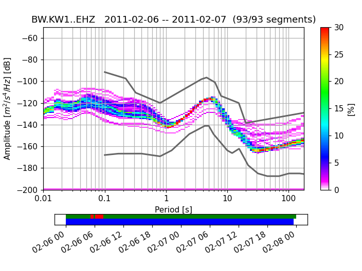
To use the colormap used by PQLX / [McNamara2004] you can import and use that
colormap from obspy.imaging.cm:
>>> from obspy.imaging.cm import pqlx
>>> ppsd.plot(cmap=pqlx)
(Source code, png)

Below the actual PPSD (for a detailed discussion see [McNamara2004]) is a visualization of the data basis for the PPSD (can also be switched off during plotting). The top row shows data fed into the PPSD, green patches represent available data, red patches represent gaps in streams that were added to the PPSD. The bottom row in blue shows the single psd measurements that go into the histogram. The default processing method fills gaps with zeros, these data segments then show up as single outlying psd lines.
Note
Providing metadata from e.g. a Dataless SEED or StationXML volume is safer
than specifying static poles and zeros information (see
PPSD).
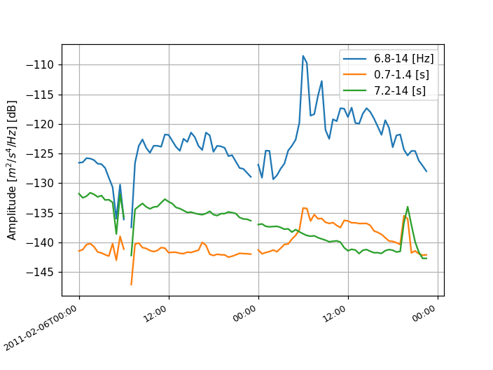
Time series of psd values can also be extracted from the PPSD by accessing the
property psd_values and
plotted using the
plot_temporal() method (temporal
restrictions can be used in the plot, see documentation):
>>> ppsd.plot_temporal([0.1, 1, 10])
(Source code, png)
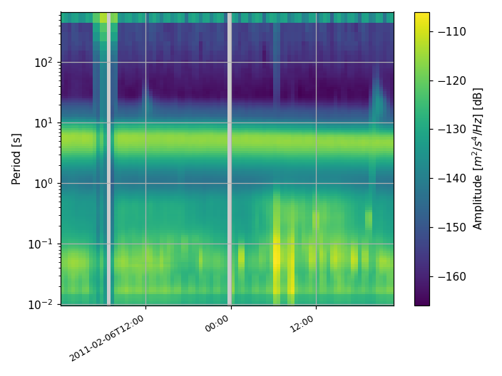
Spectrogram-like plots can be done using the
plot_spectrogram() method:
>>> ppsd.plot_spectrogram()
(Source code, png)